

148
T. Krak
satisfy ω(0) = x will furthermore satisfy ω(1) = y. Therefore, we define for the
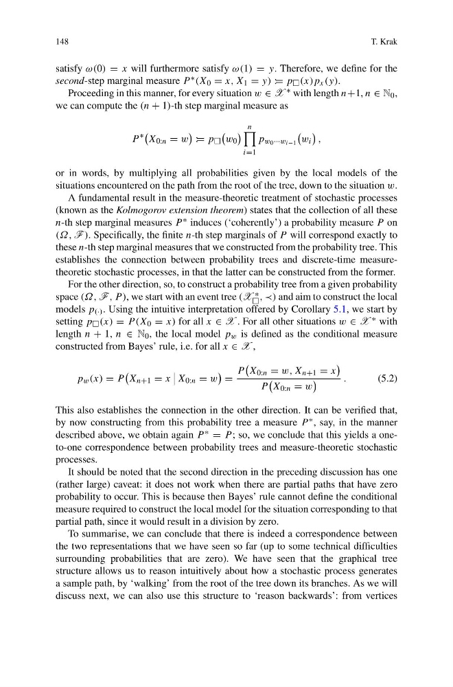
second-step marginal measure P ∗ (X 0 = x, X 1 = y) := p (x)p x (y).
Proceeding in this manner, for every situation w ∈ X ∗ with length n+1, n ∈ N 0 ,
we can compute the (n + 1)-th step marginal measure as
P
∗
X 0:n = w
:= p
w 0
n
i=1
p w 0 ···w i−1
w i
,
or in words, by multiplying all probabilities given by the local models of the
situations encountered on the path from the root of the tree, down to the situation w.
A fundamental result in the measure-theoretic treatment of stochastic processes
(known as the Kolmogorov extension theorem) states that the collection of all these
n-th step marginal measures P ∗ induces (‘coherently’) a probability measure P on
(Ω, F ). Specifically, the finite n-th step marginals of P will correspond exactly to
these n-th step marginal measures that we constructed from the probability tree. This
establishes the connection between probability trees and discrete-time measuretheoretic stochastic processes, in that the latter can be constructed from the former.
For the other direction, so, to construct a probability tree from a given probability
space (Ω, F , P ), we start with an event tree (X ∗
, ≺) and aim to construct the local
models p (·) . Using the intuitive interpretation offered by Corollary 5.1, we start by
setting p (x) = P (X 0 = x) for all x ∈ X . For all other situations w ∈ X ∗ with
length n + 1, n ∈ N 0 , the local model p w is defined as the conditional measure
constructed from Bayes’ rule, i.e. for all x ∈ X ,
p w (x) = P
X n+1 = x
X 0:n = w
=
P
X 0:n = w, X n+1 = x
P
X 0:n = w
.
(5.2)
This also establishes the connection in the other direction. It can be verified that,
by now constructing from this probability tree a measure P ∗ , say, in the manner
described above, we obtain again P ∗ = P ; so, we conclude that this yields a oneto-one correspondence between probability trees and measure-theoretic stochastic
processes.
It should be noted that the second direction in the preceding discussion has one
(rather large) caveat: it does not work when there are partial paths that have zero
probability to occur. This is because then Bayes’ rule cannot define the conditional
measure required to construct the local model for the situation corresponding to that
partial path, since it would result in a division by zero.
To summarise, we can conclude that there is indeed a correspondence between
the two representations that we have seen so far (up to some technical difficulties
surrounding probabilities that are zero). We have seen that the graphical tree
structure allows us to reason intuitively about how a stochastic process generates
a sample path, by ‘walking’ from the root of the tree down its branches. As we will
discuss next, we can also use this structure to ‘reason backwards’: from vertices
T. Krak
satisfy ω(0) = x will furthermore satisfy ω(1) = y. Therefore, we define for the
second-step marginal measure P ∗ (X 0 = x, X 1 = y) := p (x)p x (y).
Proceeding in this manner, for every situation w ∈ X ∗ with length n+1, n ∈ N 0 ,
we can compute the (n + 1)-th step marginal measure as
P
∗
X 0:n = w
:= p
w 0
n
i=1
p w 0 ···w i−1
w i
,
or in words, by multiplying all probabilities given by the local models of the
situations encountered on the path from the root of the tree, down to the situation w.
A fundamental result in the measure-theoretic treatment of stochastic processes
(known as the Kolmogorov extension theorem) states that the collection of all these
n-th step marginal measures P ∗ induces (‘coherently’) a probability measure P on
(Ω, F ). Specifically, the finite n-th step marginals of P will correspond exactly to
these n-th step marginal measures that we constructed from the probability tree. This
establishes the connection between probability trees and discrete-time measuretheoretic stochastic processes, in that the latter can be constructed from the former.
For the other direction, so, to construct a probability tree from a given probability
space (Ω, F , P ), we start with an event tree (X ∗
, ≺) and aim to construct the local
models p (·) . Using the intuitive interpretation offered by Corollary 5.1, we start by
setting p (x) = P (X 0 = x) for all x ∈ X . For all other situations w ∈ X ∗ with
length n + 1, n ∈ N 0 , the local model p w is defined as the conditional measure
constructed from Bayes’ rule, i.e. for all x ∈ X ,
p w (x) = P
X n+1 = x
X 0:n = w
=
P
X 0:n = w, X n+1 = x
P
X 0:n = w
.
(5.2)
This also establishes the connection in the other direction. It can be verified that,
by now constructing from this probability tree a measure P ∗ , say, in the manner
described above, we obtain again P ∗ = P ; so, we conclude that this yields a oneto-one correspondence between probability trees and measure-theoretic stochastic
processes.
It should be noted that the second direction in the preceding discussion has one
(rather large) caveat: it does not work when there are partial paths that have zero
probability to occur. This is because then Bayes’ rule cannot define the conditional
measure required to construct the local model for the situation corresponding to that
partial path, since it would result in a division by zero.
To summarise, we can conclude that there is indeed a correspondence between
the two representations that we have seen so far (up to some technical difficulties
surrounding probabilities that are zero). We have seen that the graphical tree
structure allows us to reason intuitively about how a stochastic process generates
a sample path, by ‘walking’ from the root of the tree down its branches. As we will
discuss next, we can also use this structure to ‘reason backwards’: from vertices