

1 Introduction to Spectral Methods for Uncertainty Quantification
9
the considered population, and it depends on the property we are looking at, on the
sampling procedure employed and on the size of the sample set.
So far we talked about characterising the population by looking at one property
at a time. Nevertheless, quite often the properties of an individual are somehow
related, like in case we were interested in characterising the population of school
students according to their age and to their height. Not surprisingly, we will likely
find out that people with a similar age will also have a similar height. Moreover, on
average the older students are also the taller ones. This means that the parameters
(age and height) are correlated, and the population is described by a joint probability
distribution of these two variables.
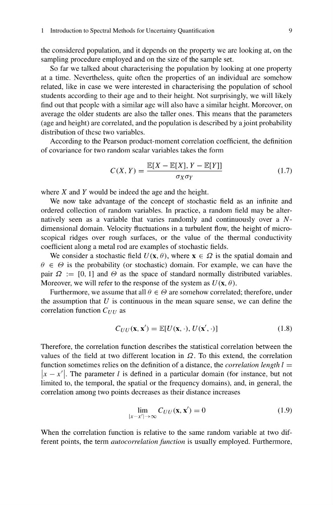
According to the Pearson product-moment correlation coefficient, the definition
of covariance for two random scalar variables takes the form
C(X, Y ) =
E[X − E[X], Y − E[Y ]]
σ X σ Y
(1.7)
where X and Y would be indeed the age and the height.
We now take advantage of the concept of stochastic field as an infinite and
ordered collection of random variables. In practice, a random field may be alternatively seen as a variable that varies randomly and continuously over a Ndimensional domain. Velocity fluctuations in a turbulent flow, the height of microscopical ridges over rough surfaces, or the value of the thermal conductivity
coefficient along a metal rod are examples of stochastic fields.
We consider a stochastic field U(x, θ), where x ∈ Ω is the spatial domain and
θ ∈ Θ is the probability (or stochastic) domain. For example, we can have the
pair Ω := [0, 1] and Θ as the space of standard normally distributed variables.
Moreover, we will refer to the response of the system as U(x, θ).
Furthermore, we assume that all θ ∈ Θ are somehow correlated; therefore, under
the assumption that U is continuous in the mean square sense, we can define the
correlation function C UU as
C UU (x, x
) = E[U(x, ·), U (x
, ·)]
(1.8)
Therefore, the correlation function describes the statistical correlation between the
values of the field at two different location in Ω. To this extend, the correlation
function sometimes relies on the definition of a distance, the correlation length l =
x − x
. The parameter l is defined in a particular domain (for instance, but not
limited to, the temporal, the spatial or the frequency domains), and, in general, the
correlation among two points decreases as their distance increases
lim
|x−x |→∞
C UU (x, x
) = 0
(1.9)
When the correlation function is relative to the same random variable at two different points, the term autocorrelation function is usually employed. Furthermore,
9
the considered population, and it depends on the property we are looking at, on the
sampling procedure employed and on the size of the sample set.
So far we talked about characterising the population by looking at one property
at a time. Nevertheless, quite often the properties of an individual are somehow
related, like in case we were interested in characterising the population of school
students according to their age and to their height. Not surprisingly, we will likely
find out that people with a similar age will also have a similar height. Moreover, on
average the older students are also the taller ones. This means that the parameters
(age and height) are correlated, and the population is described by a joint probability
distribution of these two variables.
According to the Pearson product-moment correlation coefficient, the definition
of covariance for two random scalar variables takes the form
C(X, Y ) =
E[X − E[X], Y − E[Y ]]
σ X σ Y
(1.7)
where X and Y would be indeed the age and the height.
We now take advantage of the concept of stochastic field as an infinite and
ordered collection of random variables. In practice, a random field may be alternatively seen as a variable that varies randomly and continuously over a Ndimensional domain. Velocity fluctuations in a turbulent flow, the height of microscopical ridges over rough surfaces, or the value of the thermal conductivity
coefficient along a metal rod are examples of stochastic fields.
We consider a stochastic field U(x, θ), where x ∈ Ω is the spatial domain and
θ ∈ Θ is the probability (or stochastic) domain. For example, we can have the
pair Ω := [0, 1] and Θ as the space of standard normally distributed variables.
Moreover, we will refer to the response of the system as U(x, θ).
Furthermore, we assume that all θ ∈ Θ are somehow correlated; therefore, under
the assumption that U is continuous in the mean square sense, we can define the
correlation function C UU as
C UU (x, x
) = E[U(x, ·), U (x
, ·)]
(1.8)
Therefore, the correlation function describes the statistical correlation between the
values of the field at two different location in Ω. To this extend, the correlation
function sometimes relies on the definition of a distance, the correlation length l =
x − x
. The parameter l is defined in a particular domain (for instance, but not
limited to, the temporal, the spatial or the frequency domains), and, in general, the
correlation among two points decreases as their distance increases
lim
|x−x |→∞
C UU (x, x
) = 0
(1.9)
When the correlation function is relative to the same random variable at two different points, the term autocorrelation function is usually employed. Furthermore,