

116
D. Krpelík et al.
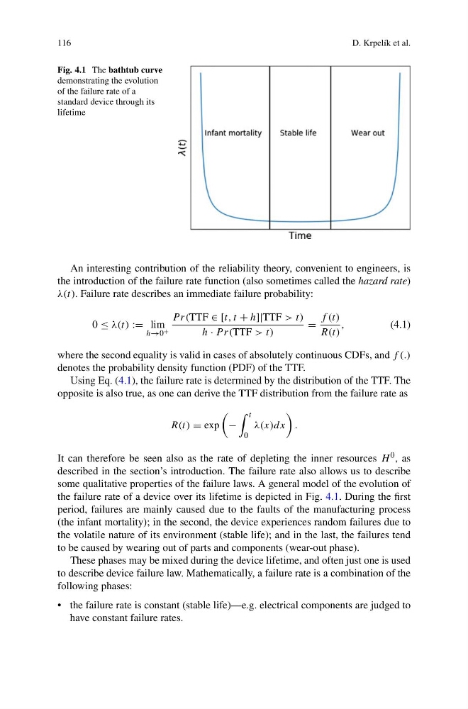
Fig. 4.1 The bathtub curve
demonstrating the evolution
of the failure rate of a
standard device through its
lifetime
An interesting contribution of the reliability theory, convenient to engineers, is
the introduction of the failure rate function (also sometimes called the hazard rate)
λ(t). Failure rate describes an immediate failure probability:
0 ≤ λ(t) := lim
h→0 +
P r(TTF ∈ [t, t + h]|TTF > t)
h · P r(TTF > t)
=
f (t)
R(t)
,
(4.1)
where the second equality is valid in cases of absolutely continuous CDFs, and f (.)
denotes the probability density function (PDF) of the TTF.
Using Eq. (4.1), the failure rate is determined by the distribution of the TTF. The
opposite is also true, as one can derive the TTF distribution from the failure rate as
R(t) = exp
−
t
0
λ(x)dx
.
It can therefore be seen also as the rate of depleting the inner resources H 0 , as
described in the section’s introduction. The failure rate also allows us to describe
some qualitative properties of the failure laws. A general model of the evolution of
the failure rate of a device over its lifetime is depicted in Fig. 4.1. During the first
period, failures are mainly caused due to the faults of the manufacturing process
(the infant mortality); in the second, the device experiences random failures due to
the volatile nature of its environment (stable life); and in the last, the failures tend
to be caused by wearing out of parts and components (wear-out phase).
These phases may be mixed during the device lifetime, and often just one is used
to describe device failure law. Mathematically, a failure rate is a combination of the
following phases:
• the failure rate is constant (stable life)—e.g. electrical components are judged to
have constant failure rates.
D. Krpelík et al.
Fig. 4.1 The bathtub curve
demonstrating the evolution
of the failure rate of a
standard device through its
lifetime
An interesting contribution of the reliability theory, convenient to engineers, is
the introduction of the failure rate function (also sometimes called the hazard rate)
λ(t). Failure rate describes an immediate failure probability:
0 ≤ λ(t) := lim
h→0 +
P r(TTF ∈ [t, t + h]|TTF > t)
h · P r(TTF > t)
=
f (t)
R(t)
,
(4.1)
where the second equality is valid in cases of absolutely continuous CDFs, and f (.)
denotes the probability density function (PDF) of the TTF.
Using Eq. (4.1), the failure rate is determined by the distribution of the TTF. The
opposite is also true, as one can derive the TTF distribution from the failure rate as
R(t) = exp
−
t
0
λ(x)dx
.
It can therefore be seen also as the rate of depleting the inner resources H 0 , as
described in the section’s introduction. The failure rate also allows us to describe
some qualitative properties of the failure laws. A general model of the evolution of
the failure rate of a device over its lifetime is depicted in Fig. 4.1. During the first
period, failures are mainly caused due to the faults of the manufacturing process
(the infant mortality); in the second, the device experiences random failures due to
the volatile nature of its environment (stable life); and in the last, the failures tend
to be caused by wearing out of parts and components (wear-out phase).
These phases may be mixed during the device lifetime, and often just one is used
to describe device failure law. Mathematically, a failure rate is a combination of the
following phases:
• the failure rate is constant (stable life)—e.g. electrical components are judged to
have constant failure rates.