

3 Uncertainty Quantification in Lasso-Type Regularization Problems
97
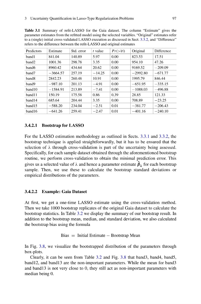
Table 3.1 Summary of refit-LASSO for the Gaia dataset. The column “Estimate” gives the
parameter estimates from the refitted model using the selected variables. “Original” estimates refer
to a (single) initial cross-validated LASSO execution as discussed in Sect. 3.3.2, and “Difference”
refers to the difference between the refit-LASSO and original estimates
Predictors
Estimate
Std. error
t value
P r(>|t|)
Original
Difference
band1
841.04
140.89
5.97
0.00
823.53
17.51
band2
1001.36
298.78
3.35
0.00
954.10
47.26
band6
8960.42
434.64
20.62
0.00
9169.52
−209.09
band7
−3664.57
257.19
−14.25
0.00
−2992.80
−671.77
band8
2842.23
260.48
10.91
0.00
1995.79
846.44
band9
−987.10
201.13
−4.91
0.00
−651.95
−335.15
band10
−1584.91
213.89
−7.41
0.00
−1088.03
−496.88
band11
150.19
175.58
0.86
0.39
28.85
121.33
band14
685.64
204.44
3.35
0.00
708.89
−23.25
band15
−588.20
234.04
−2.51
0.01
−381.77
−206.43
band16
−641.26
259.41
−2.47
0.01
−401.16
−240.10
3.4.2.1 Bootstrap for LASSO
For the LASSO estimation methodology as outlined in Sects. 3.3.1 and 3.3.2, the
bootstrap technique is applied straightforwardly, but it has to be ensured that the
selection of λ through cross-validation is part of the uncertainty being assessed.
Specifically, for each sample dataset obtained through the aforementioned bootstrap
routine, we perform cross-validation to obtain the minimal prediction error. This
gives us a selected value of λ and hence a parameter estimate ˆ
β λ for each bootstrap
sample. Then, we use these to calculate the bootstrap standard deviations or
empirical distributions of the parameters.
3.4.2.2 Example: Gaia Dataset
At first, we get a one-time LASSO estimate using the cross-validation method.
Then we take 1000 bootstrap replicates of the original Gaia dataset to calculate the
bootstrap statistics. In Table 3.2 we display the summary of our bootstrap result. In
addition to the bootstrap mean, median, and standard deviation, we also calculated
the bootstrap bias using the formula
Bias = Initial Estimate − Bootstrap Mean
In Fig. 3.8, we visualize the bootstrapped distribution of the parameters through
box-plots.
Clearly, it can be seen from Table 3.2 and Fig. 3.8 that band3, band4, band5,
band12, and band13 are the non-important parameters. While the mean for band3
and band13 is not very close to 0, they still act as non-important parameters with
median being 0.
97
Table 3.1 Summary of refit-LASSO for the Gaia dataset. The column “Estimate” gives the
parameter estimates from the refitted model using the selected variables. “Original” estimates refer
to a (single) initial cross-validated LASSO execution as discussed in Sect. 3.3.2, and “Difference”
refers to the difference between the refit-LASSO and original estimates
Predictors
Estimate
Std. error
t value
P r(>|t|)
Original
Difference
band1
841.04
140.89
5.97
0.00
823.53
17.51
band2
1001.36
298.78
3.35
0.00
954.10
47.26
band6
8960.42
434.64
20.62
0.00
9169.52
−209.09
band7
−3664.57
257.19
−14.25
0.00
−2992.80
−671.77
band8
2842.23
260.48
10.91
0.00
1995.79
846.44
band9
−987.10
201.13
−4.91
0.00
−651.95
−335.15
band10
−1584.91
213.89
−7.41
0.00
−1088.03
−496.88
band11
150.19
175.58
0.86
0.39
28.85
121.33
band14
685.64
204.44
3.35
0.00
708.89
−23.25
band15
−588.20
234.04
−2.51
0.01
−381.77
−206.43
band16
−641.26
259.41
−2.47
0.01
−401.16
−240.10
3.4.2.1 Bootstrap for LASSO
For the LASSO estimation methodology as outlined in Sects. 3.3.1 and 3.3.2, the
bootstrap technique is applied straightforwardly, but it has to be ensured that the
selection of λ through cross-validation is part of the uncertainty being assessed.
Specifically, for each sample dataset obtained through the aforementioned bootstrap
routine, we perform cross-validation to obtain the minimal prediction error. This
gives us a selected value of λ and hence a parameter estimate ˆ
β λ for each bootstrap
sample. Then, we use these to calculate the bootstrap standard deviations or
empirical distributions of the parameters.
3.4.2.2 Example: Gaia Dataset
At first, we get a one-time LASSO estimate using the cross-validation method.
Then we take 1000 bootstrap replicates of the original Gaia dataset to calculate the
bootstrap statistics. In Table 3.2 we display the summary of our bootstrap result. In
addition to the bootstrap mean, median, and standard deviation, we also calculated
the bootstrap bias using the formula
Bias = Initial Estimate − Bootstrap Mean
In Fig. 3.8, we visualize the bootstrapped distribution of the parameters through
box-plots.
Clearly, it can be seen from Table 3.2 and Fig. 3.8 that band3, band4, band5,
band12, and band13 are the non-important parameters. While the mean for band3
and band13 is not very close to 0, they still act as non-important parameters with
median being 0.