

600
E. Fernández et al.
carrying out production activities related to new and returned products. Given the
computational complexity to solve a MILP of a production system that involves
capacity constraints and return options (Bitran and Yanasse 1982; Retel-Helmrich
et al. 2014), for the numerical experimentation we consider only the information of
a certain period of time that is representative and that resulted in a planning horizon
of T = 21. In the case of the model for the hybrid system, we add a new family of
constraints for considering only those solutions for which the inspection of returns in
certain period involve all the available returns of the same quality. The convenience
of this decision is supported by the findings of (Devoto et al. 2019) over a hybrid
system of a single item. In addition, the safety stock level of final products was
estimated as one third of the level of the current production system without returns,
since in the hybrid system there are three different production lines of products (one
for new products and two for remanufacturable products).
The values of the parameters used in this study for both models were estimated
based on historical data of the firm. Returns were estimated as the 60% of the demand
values. Models were coded in AMPL and solved with solver Gurobi 8.1.0 on a PC
with Windows 10, CPU i7-4710HQ, 2.50 GHz and 16 Gb of RAM. The running
time of the solver was limited to 17 h, since in the 5 h after the first 12 h of execution
there was no substantial improvement in the quality of the solution (less than 0.09%
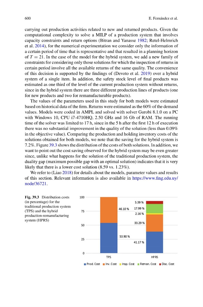
in the objective value). Comparing the production and holding inventory costs of the
solutions obtained for both models, we note that the saving for the hybrid system is
7.2%. Figure 39.3 shows the distribution of the costs of both solutions. In addition, we
want to point out the cost saving observed for the hybrid system may be even greater
since, unlike what happens for the solution of the traditional production system, the
duality gap (maximum possible gap with an optimal solution) indicates that it is very
likely that there is a lower cost solution (8.59 vs. 1.23%).
We refer to (Liao 2018) for details about the models, parameter values and results
of this section. Relevant information is also available in https://www.fing.edu.uy/
node/36721.
Fig. 39.3 Distribution costs
(in percentage) for the
traditional production system
(TPS) and the hybrid
production-remanufacturing
system (HPRS)