

338
5 X-ray Pulsar-Based Navigation: Theories and Experiments
For this way, an infinite dimensional power spectrum estimation S m is obtained.
Similar to the method usually used in the Allan variance, the S m is divided by the
third power exponent of time, and thus an infinite dimensional Sigma-z variance is
obtained, i.e.,
σ
2
z (τ ) =
1
τ 3 S m ,
(5.92)
where τ =
1
m
T .
This is the original algorithm of the Sigma-z variance proposed by Joseph H.
Taylor. The Sigma-z variance σ
2
z (τ ) obeys the chi-square distribution with the degree
of freedom of m. This variance statistical method is applicable to the processing of
non-equal-interval and discontinuous pulsar timing observation data. Of course, it is
also applicable to the analyzing and processing of the stability of atomic clock with
equal interval measurement data.
In addition, by directly using the pulsar timing residual measurement data to fit a
third-order polynomial function, an improved Sigma-z variance statistical algorithm
was proposed by Matsakis et al. in 1997 [26]. Similarly, the time residual sequence
is divided into m subsequences (m = 1, 2, 4, 8, …), and then the residual data of
each subsequence is used for the least squares fitting, so as to meet
R
2
=
N m
i=1
x(t i ) −
X (t i )
σ i
2
= min,
(5.93)
where X (t i ) = c 0 +c 1 (t i − t 0 )+c 2 (t i − t 0 )
2
+c 3 (t i − t 0 )
3 ; x(t i ) is the phase measurement residual of time; σ i is the uncertainty of time measurement; t i is the observational
time; t 0 is the arbitrarily selected deviation time; N m is the measurement number for
the subsequence.
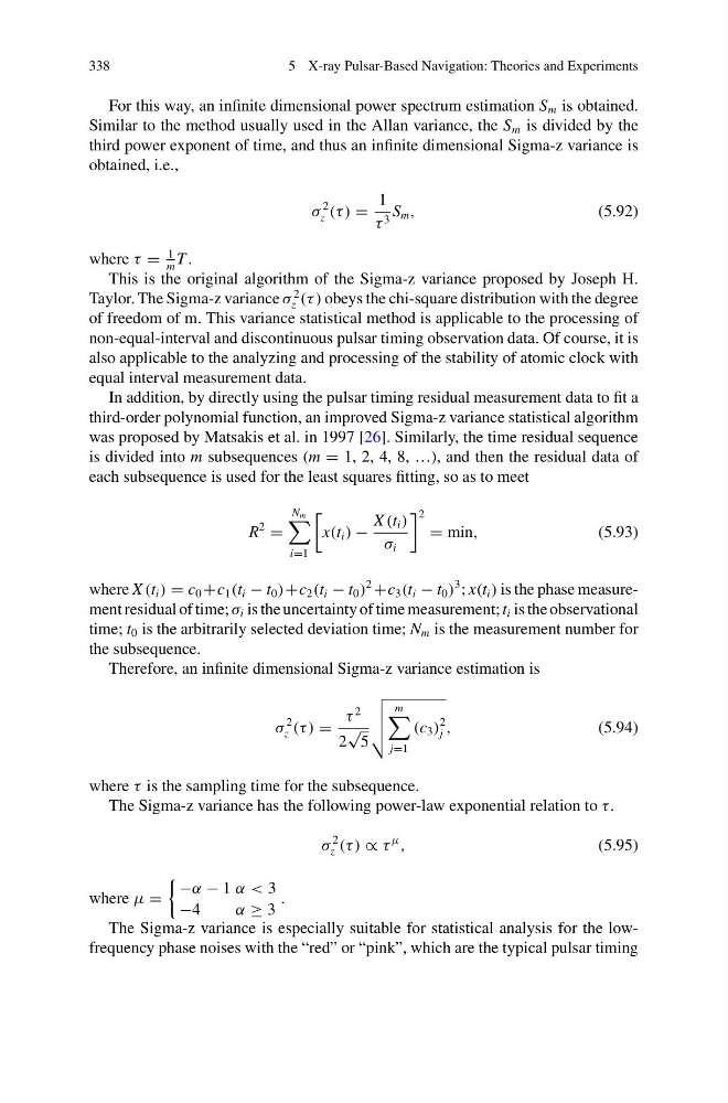
Therefore, an infinite dimensional Sigma-z variance estimation is
σ
2
z (τ ) =
τ
2
2
√
5
m
j=1
(c 3 )
2
j ,
(5.94)
where τ is the sampling time for the subsequence.
The Sigma-z variance has the following power-law exponential relation to τ.
σ
2
z (τ ) ∝ τ
μ
,
(5.95)
where μ =
−α − 1 α < 3
−4
α ≥ 3
.
The Sigma-z variance is especially suitable for statistical analysis for the lowfrequency phase noises with the “red” or “pink”, which are the typical pulsar timing
5 X-ray Pulsar-Based Navigation: Theories and Experiments
For this way, an infinite dimensional power spectrum estimation S m is obtained.
Similar to the method usually used in the Allan variance, the S m is divided by the
third power exponent of time, and thus an infinite dimensional Sigma-z variance is
obtained, i.e.,
σ
2
z (τ ) =
1
τ 3 S m ,
(5.92)
where τ =
1
m
T .
This is the original algorithm of the Sigma-z variance proposed by Joseph H.
Taylor. The Sigma-z variance σ
2
z (τ ) obeys the chi-square distribution with the degree
of freedom of m. This variance statistical method is applicable to the processing of
non-equal-interval and discontinuous pulsar timing observation data. Of course, it is
also applicable to the analyzing and processing of the stability of atomic clock with
equal interval measurement data.
In addition, by directly using the pulsar timing residual measurement data to fit a
third-order polynomial function, an improved Sigma-z variance statistical algorithm
was proposed by Matsakis et al. in 1997 [26]. Similarly, the time residual sequence
is divided into m subsequences (m = 1, 2, 4, 8, …), and then the residual data of
each subsequence is used for the least squares fitting, so as to meet
R
2
=
N m
i=1
x(t i ) −
X (t i )
σ i
2
= min,
(5.93)
where X (t i ) = c 0 +c 1 (t i − t 0 )+c 2 (t i − t 0 )
2
+c 3 (t i − t 0 )
3 ; x(t i ) is the phase measurement residual of time; σ i is the uncertainty of time measurement; t i is the observational
time; t 0 is the arbitrarily selected deviation time; N m is the measurement number for
the subsequence.
Therefore, an infinite dimensional Sigma-z variance estimation is
σ
2
z (τ ) =
τ
2
2
√
5
m
j=1
(c 3 )
2
j ,
(5.94)
where τ is the sampling time for the subsequence.
The Sigma-z variance has the following power-law exponential relation to τ.
σ
2
z (τ ) ∝ τ
μ
,
(5.95)
where μ =
−α − 1 α < 3
−4
α ≥ 3
.
The Sigma-z variance is especially suitable for statistical analysis for the lowfrequency phase noises with the “red” or “pink”, which are the typical pulsar timing