

6
1 Essentials of Non-relativistic Two-Body Scattering Theory
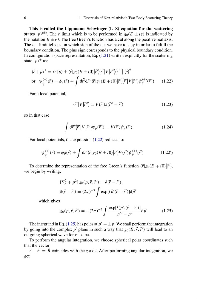
This is called the Lippmann–Schwinger (L–S) equation for the scattering
states | p
(±) . The ε limit which is to be performed in g 0 (E ± iε) is indicated by
the notation E ± i0. The free Green’s function has a cut along the positive real axis.
The ε− limit tells us on which side of the cut we have to stay in order to fulfill the
boundary condition. The plus sign corresponds to the physical boundary condition.
In configuration space representation, Eq. (1.21) written explicitly for the scattering
state | p
+ as:
r |
p
+ = r | p + r |g 0 (E + i0)
r
r
V
r
r
p
+
or ψ
(+)
p
( r ) = φ
p ( r ) +
d
r d r
r |g 0 (E + i0)
r
r
V
r
ψ
(+)
p ( r
)
(1.22)
For a local potential,
r
V
r
= V ( r
)δ( r
− −
r
)
(1.23)
so in that case
d r
r
V
r
ψ p ( r
) = V ( r
)ψ
p ( r
)
(1.24)
For local potentials, the expression (1.22) reduces to:
ψ
(+)
p
( r ) = φ
p ( r ) +
d r
r |g 0 (E + i0)
r
V ( r
)ψ
(+)
p ( r
)
(1.22
)
To determine the representation of the free Green’s function r |g 0 (E + i0)
r
,
we begin by writing:
[∇
2
r + p
2
] g 0 ( p,
r ,
r
) = δ( r − −
r
),
δ( r − −
r
) = (2π)
−3
exp[i
p
( r − −
r
)]d
p
which gives
g 0 ( p,
r ,
r
) = −(2π)
−3
exp[i(
p
.( r − −
r
)]
p 2 − p 2
d
p
(1.25)
The integrand in Eq. (1.25) has poles at p
= ±p. We shall perform the integration
by going into the complex p
plane in such a way that g 0 (E,
r ,
r
) will lead to an
outgoing spherical wave for r → ∞.
To perform the angular integration, we choose spherical polar coordinates such
that the vector
r − −
r
≡
R coincides with the z-axis. After performing angular integration, we
get
1 Essentials of Non-relativistic Two-Body Scattering Theory
This is called the Lippmann–Schwinger (L–S) equation for the scattering
states | p
(±) . The ε limit which is to be performed in g 0 (E ± iε) is indicated by
the notation E ± i0. The free Green’s function has a cut along the positive real axis.
The ε− limit tells us on which side of the cut we have to stay in order to fulfill the
boundary condition. The plus sign corresponds to the physical boundary condition.
In configuration space representation, Eq. (1.21) written explicitly for the scattering
state | p
+ as:
r |
p
+ = r | p + r |g 0 (E + i0)
r
r
V
r
r
p
+
or ψ
(+)
p
( r ) = φ
p ( r ) +
d
r d r
r |g 0 (E + i0)
r
r
V
r
ψ
(+)
p ( r
)
(1.22)
For a local potential,
r
V
r
= V ( r
)δ( r
− −
r
)
(1.23)
so in that case
d r
r
V
r
ψ p ( r
) = V ( r
)ψ
p ( r
)
(1.24)
For local potentials, the expression (1.22) reduces to:
ψ
(+)
p
( r ) = φ
p ( r ) +
d r
r |g 0 (E + i0)
r
V ( r
)ψ
(+)
p ( r
)
(1.22
)
To determine the representation of the free Green’s function r |g 0 (E + i0)
r
,
we begin by writing:
[∇
2
r + p
2
] g 0 ( p,
r ,
r
) = δ( r − −
r
),
δ( r − −
r
) = (2π)
−3
exp[i
p
( r − −
r
)]d
p
which gives
g 0 ( p,
r ,
r
) = −(2π)
−3
exp[i(
p
.( r − −
r
)]
p 2 − p 2
d
p
(1.25)
The integrand in Eq. (1.25) has poles at p
= ±p. We shall perform the integration
by going into the complex p
plane in such a way that g 0 (E,
r ,
r
) will lead to an
outgoing spherical wave for r → ∞.
To perform the angular integration, we choose spherical polar coordinates such
that the vector
r − −
r
≡
R coincides with the z-axis. After performing angular integration, we
get