

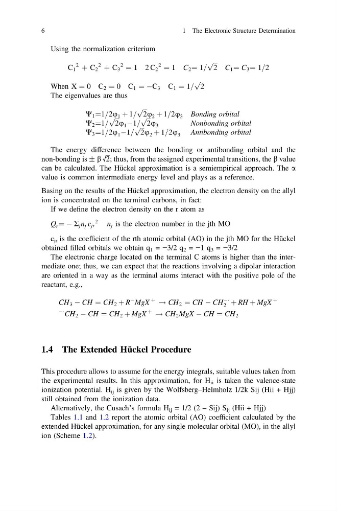
Using the normalization criterium
C 1
2
þ C 2
2
þ C 3
2
¼ 1 2C 2
2
¼ 1 C 2 ¼ 1=
ffiffi ffi
2
p
C 1 ¼ C 3 ¼ 1=2
When X ¼ 0 C 2 ¼ 0 C 1 ¼ ÀC 3 C 1 ¼ 1=
ffiffi ffi
2
p
The eigenvalues are thus
W 1 ¼1=2u 1 þ 1=
ffiffi ffi
2
p u 2 þ 1=2u 3 Bonding orbital
W 2 ¼1=
ffiffi ffi
2
p u 1 À1=
ffiffi ffi
2
p u 3
Nonbonding orbital
W 3 ¼1=2u 1 À1=
ffiffi ffi
2
p u 2 þ 1=2u 3 Antibonding orbital
The energy difference between the bonding or antibonding orbital and the
non-bonding is ± b √2; thus, from the assigned experimental transitions, the b value
can be calculated. The Hückel approximation is a semiempirical approach. The a
value is common intermediate energy level and plays as a reference.
Basing on the results of the Hückel approximation, the electron density on the allyl
ion is concentrated on the terminal carbons, in fact:
If we define the electron density on the r atom as
Q r ¼ À R j n j c jr
2
n j is the electron number in the jth MO
c jr is the coefficient of the rth atomic orbital (AO) in the jth MO for the Hückel
obtained filled orbitals we obtain q 1 = −3/2 q 2 = −1 q 3 = −3/2
The electronic charge located on the terminal C atoms is higher than the intermediate one; thus, we can expect that the reactions involving a dipolar interaction
are oriented in a way as the terminal atoms interact with the positive pole of the
reactant, e.g.,
CH 3 À CH ¼ CH 2 þ R
À MgX
þ
! CH 2 ¼ CH À CH
ÀÁ
2 þ RH þ MgX
þ
ÀÁ CH 2 À CH ¼ CH 2 þ MgX
þ
! CH 2 MgX À CH ¼ CH 2
1.4 The Extended Hückel Procedure
This procedure allows to assume for the energy integrals, suitable values taken from
the experimental results. In this approximation, for H ii is taken the valence-state
ionization potential. H ij is given by the Wolfsberg–Helmholz 1/2k Sij (Hii + Hjj)
still obtained from the ionization data.
Alternatively, the Cusach’s formula H ij = 1/2 (2 – Sij) S ij (Hii + Hjj)
Tables 1.1 and 1.2 report the atomic orbital (AO) coefficient calculated by the
extended Hückel approximation, for any single molecular orbital (MO), in the allyl
ion (Scheme 1.2).
6
1 The Electronic Structure Determination
C 1
2
þ C 2
2
þ C 3
2
¼ 1 2C 2
2
¼ 1 C 2 ¼ 1=
ffiffi ffi
2
p
C 1 ¼ C 3 ¼ 1=2
When X ¼ 0 C 2 ¼ 0 C 1 ¼ ÀC 3 C 1 ¼ 1=
ffiffi ffi
2
p
The eigenvalues are thus
W 1 ¼1=2u 1 þ 1=
ffiffi ffi
2
p u 2 þ 1=2u 3 Bonding orbital
W 2 ¼1=
ffiffi ffi
2
p u 1 À1=
ffiffi ffi
2
p u 3
Nonbonding orbital
W 3 ¼1=2u 1 À1=
ffiffi ffi
2
p u 2 þ 1=2u 3 Antibonding orbital
The energy difference between the bonding or antibonding orbital and the
non-bonding is ± b √2; thus, from the assigned experimental transitions, the b value
can be calculated. The Hückel approximation is a semiempirical approach. The a
value is common intermediate energy level and plays as a reference.
Basing on the results of the Hückel approximation, the electron density on the allyl
ion is concentrated on the terminal carbons, in fact:
If we define the electron density on the r atom as
Q r ¼ À R j n j c jr
2
n j is the electron number in the jth MO
c jr is the coefficient of the rth atomic orbital (AO) in the jth MO for the Hückel
obtained filled orbitals we obtain q 1 = −3/2 q 2 = −1 q 3 = −3/2
The electronic charge located on the terminal C atoms is higher than the intermediate one; thus, we can expect that the reactions involving a dipolar interaction
are oriented in a way as the terminal atoms interact with the positive pole of the
reactant, e.g.,
CH 3 À CH ¼ CH 2 þ R
À MgX
þ
! CH 2 ¼ CH À CH
ÀÁ
2 þ RH þ MgX
þ
ÀÁ CH 2 À CH ¼ CH 2 þ MgX
þ
! CH 2 MgX À CH ¼ CH 2
1.4 The Extended Hückel Procedure
This procedure allows to assume for the energy integrals, suitable values taken from
the experimental results. In this approximation, for H ii is taken the valence-state
ionization potential. H ij is given by the Wolfsberg–Helmholz 1/2k Sij (Hii + Hjj)
still obtained from the ionization data.
Alternatively, the Cusach’s formula H ij = 1/2 (2 – Sij) S ij (Hii + Hjj)
Tables 1.1 and 1.2 report the atomic orbital (AO) coefficient calculated by the
extended Hückel approximation, for any single molecular orbital (MO), in the allyl
ion (Scheme 1.2).
6
1 The Electronic Structure Determination