

E1C11 09/14/2010
13:14:3 Page 482
In practical applications, it is most often the case that changes in resistance are small in
comparison to the resistance values, that is, dR=R ( 1; thus
dE 0
E i
¼
dR 1 =R 1
ð
Þ 1 þ y p
À
Á
4
ð11:28Þ
Therefore the bridge constant is the ratio of Equation 11.28 to Equation 11.14:
dR 1 =R 1
ð
Þ 1 þ y p
À
Á =4
dR 1 =R 1
ð
Þ =4
ð11:29Þ
And the bridge constant is
k ¼ 1 þ y p
Comparing Equation 11.28 to Equation 11.14 shows that the use of two gauges oriented as
described has increased the output of the bridge by a factor of 1 þ y p over that of using a single
gauge.
11.6 APPARENT STRAIN AND TEMPERATURE COMPENSATION
Apparent strain is manifested as any change in gauge resistance that is not due to the component of
strain being measured. Techniques for accomplishing temperature compensation, eliminating
certain components of strain, and increasing the value of the bridge constant can be devised by
examining more closely Equation 11.22. The bridge constant is influenced by (1) the location of
strain gauges on the test specimen and (2) the gauge connection positions in the bridge circuit. The
combined effect of these two factors is determined by examining the existing strain field and using
Equation 11.22 to determine the resulting bridge output.
Let us examine how a component of strain can be removed (compensation) from the measured
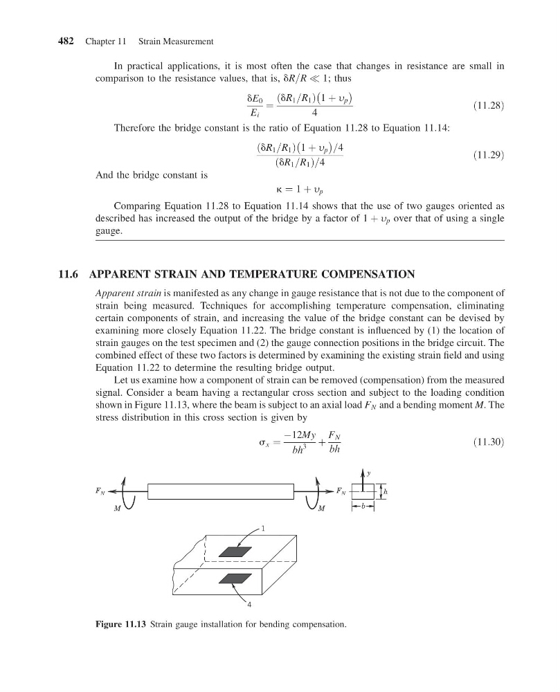
signal. Consider a beam having a rectangular cross section and subject to the loading condition
shown in Figure 11.13, where the beam is subject to an axial load F N and a bending moment M. The
stress distribution in this cross section is given by
s x ¼
À12My
bh
3
þ
F N
bh
ð11:30Þ
1
4
F N
F N
h
y
M
M
b
Figure 11.13 Strain gauge installation for bending compensation.
482 Chapter 11 Strain Measurement
13:14:3 Page 482
In practical applications, it is most often the case that changes in resistance are small in
comparison to the resistance values, that is, dR=R ( 1; thus
dE 0
E i
¼
dR 1 =R 1
ð
Þ 1 þ y p
À
Á
4
ð11:28Þ
Therefore the bridge constant is the ratio of Equation 11.28 to Equation 11.14:
dR 1 =R 1
ð
Þ 1 þ y p
À
Á =4
dR 1 =R 1
ð
Þ =4
ð11:29Þ
And the bridge constant is
k ¼ 1 þ y p
Comparing Equation 11.28 to Equation 11.14 shows that the use of two gauges oriented as
described has increased the output of the bridge by a factor of 1 þ y p over that of using a single
gauge.
11.6 APPARENT STRAIN AND TEMPERATURE COMPENSATION
Apparent strain is manifested as any change in gauge resistance that is not due to the component of
strain being measured. Techniques for accomplishing temperature compensation, eliminating
certain components of strain, and increasing the value of the bridge constant can be devised by
examining more closely Equation 11.22. The bridge constant is influenced by (1) the location of
strain gauges on the test specimen and (2) the gauge connection positions in the bridge circuit. The
combined effect of these two factors is determined by examining the existing strain field and using
Equation 11.22 to determine the resulting bridge output.
Let us examine how a component of strain can be removed (compensation) from the measured
signal. Consider a beam having a rectangular cross section and subject to the loading condition
shown in Figure 11.13, where the beam is subject to an axial load F N and a bending moment M. The
stress distribution in this cross section is given by
s x ¼
À12My
bh
3
þ
F N
bh
ð11:30Þ
1
4
F N
F N
h
y
M
M
b
Figure 11.13 Strain gauge installation for bending compensation.
482 Chapter 11 Strain Measurement