

E1C04 09/14/2010
14:7:44 Page 145
The random uncertainty between the data and this fit is given by the standard error of the fit, s yx .
Using Equation 4.35,
s yx ¼
ffiffiffiffiffiffiffiffiffiffiffiffiffiffiffiffiffiffiffiffiffiffiffiffiffiffiffiffiffiffiffiffi
P N
i¼1 y i À y c i
À
Á 2
n
s
¼ 0:16
with degrees of freedom, n ¼ N À m þ 1
ð
Þ¼3. The t estimator, t 3,95 ¼ 3.18, establishes a random
uncertainty about the fit of t 3;95 s yx =
ffiffiffiffi
N
p ¼ 0:23. Applying Equation 4.39, the polynomial fit can be
stated at 95% confidence as
y c ¼ 1:04x þ 0:02 Æ 0:23 V 95%
ð
Þ
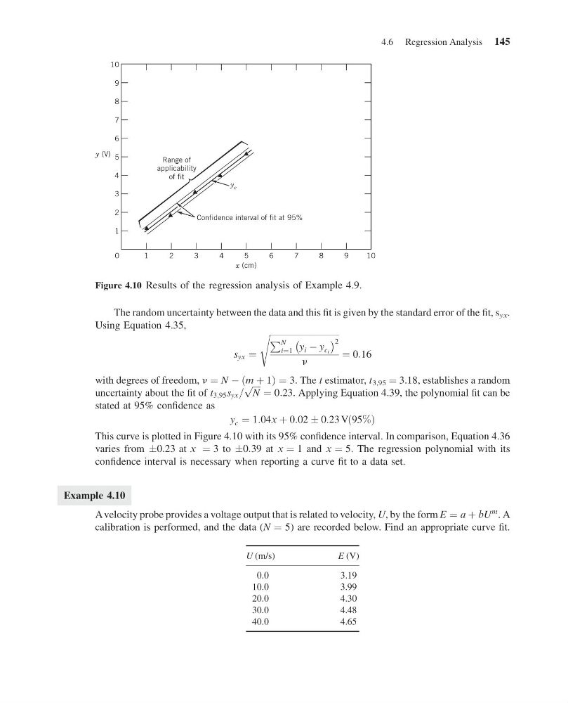
This curve is plotted in Figure 4.10 with its 95% confidence interval. In comparison, Equation 4.36
varies from Æ0:23 at x ¼ 3 to Æ0:39 at x ¼ 1 and x ¼ 5. The regression polynomial with its
confidence interval is necessary when reporting a curve fit to a data set.
Example 4.10
A velocity probe provides a voltage output that is related to velocity, U, by the form E ¼ a þ bU
m . A
calibration is performed, and the data (N ¼ 5) are recorded below. Find an appropriate curve fit.
U (m/s)
E (V)
0.0
3.19
10.0
3.99
20.0
4.30
30.0
4.48
40.0
4.65
0
1
2
3
Confidence interval of fit at 95%
Range of
applicability
of fit
4
5
6
7
8
9
1 0
y (V)
x (cm)
1
2
3
4
5
6
7
8
9
10
y c
Figure 4.10 Results of the regression analysis of Example 4.9.
4.6 Regression Analysis 145
14:7:44 Page 145
The random uncertainty between the data and this fit is given by the standard error of the fit, s yx .
Using Equation 4.35,
s yx ¼
ffiffiffiffiffiffiffiffiffiffiffiffiffiffiffiffiffiffiffiffiffiffiffiffiffiffiffiffiffiffiffiffi
P N
i¼1 y i À y c i
À
Á 2
n
s
¼ 0:16
with degrees of freedom, n ¼ N À m þ 1
ð
Þ¼3. The t estimator, t 3,95 ¼ 3.18, establishes a random
uncertainty about the fit of t 3;95 s yx =
ffiffiffiffi
N
p ¼ 0:23. Applying Equation 4.39, the polynomial fit can be
stated at 95% confidence as
y c ¼ 1:04x þ 0:02 Æ 0:23 V 95%
ð
Þ
This curve is plotted in Figure 4.10 with its 95% confidence interval. In comparison, Equation 4.36
varies from Æ0:23 at x ¼ 3 to Æ0:39 at x ¼ 1 and x ¼ 5. The regression polynomial with its
confidence interval is necessary when reporting a curve fit to a data set.
Example 4.10
A velocity probe provides a voltage output that is related to velocity, U, by the form E ¼ a þ bU
m . A
calibration is performed, and the data (N ¼ 5) are recorded below. Find an appropriate curve fit.
U (m/s)
E (V)
0.0
3.19
10.0
3.99
20.0
4.30
30.0
4.48
40.0
4.65
0
1
2
3
Confidence interval of fit at 95%
Range of
applicability
of fit
4
5
6
7
8
9
1 0
y (V)
x (cm)
1
2
3
4
5
6
7
8
9
10
y c
Figure 4.10 Results of the regression analysis of Example 4.9.
4.6 Regression Analysis 145