

E1C04 09/14/2010
14:7:43 Page 142
The best order of polynomial fit to apply to a particular data set is that lowest order of fit that
maintains a logical physical sense between the dependent and independent variables and reduces s yx
to an acceptable value. This first point is important. If the underlying physics of a problem implies
that a certain order relationship should exist between dependent and independent variables, there is
no sense in forcing the data to fit any other order of polynomial regardless of the value of s yx .
Because the method of least-squares tries to minimize the sum of the squares of the deviations, it
forces inflections in the curve fit that may not be real. Consequently, while higher-order curve fits
generally reduce s yx , they likely do not reflect the physics behind the data set very well. In any event,
it is good practice to have at least two independent data points for each order of polynomial
attempted, that is, at least two data points for a first-order curve fit, four for a second-order, etc.
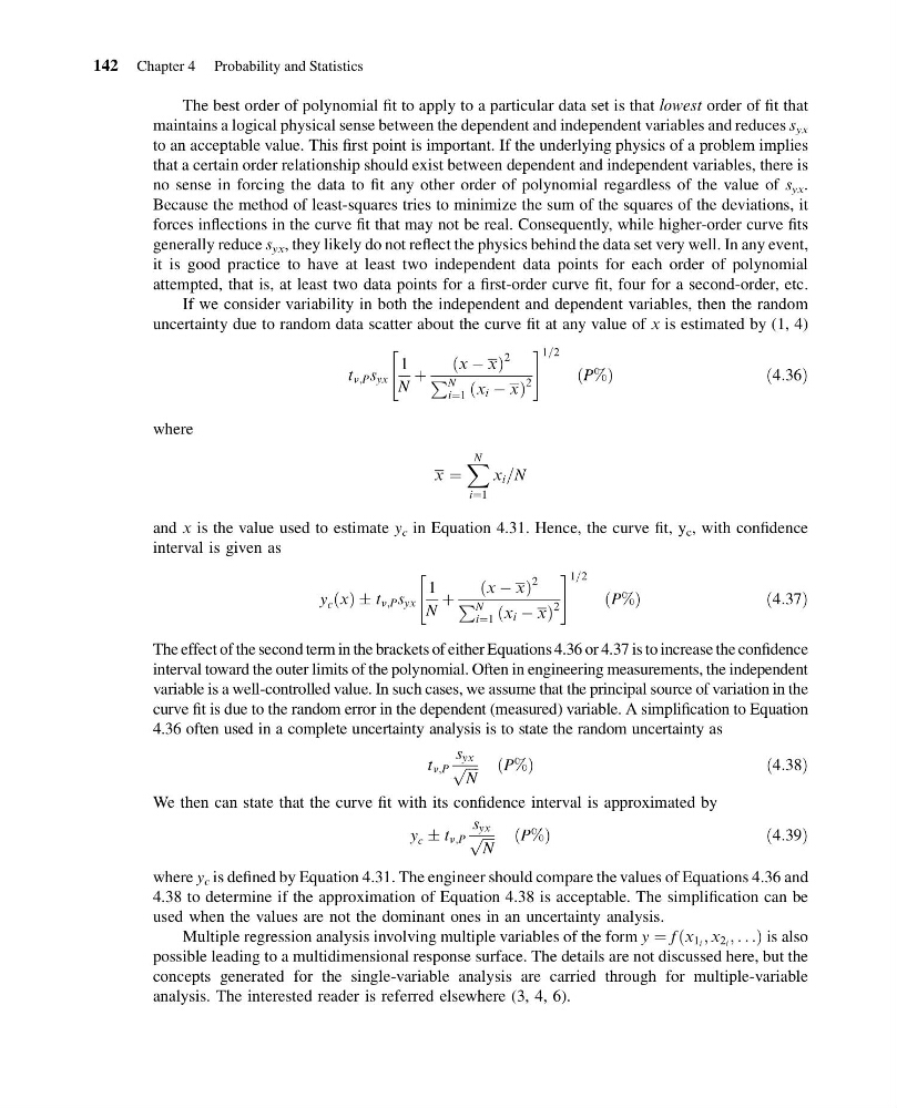
If we consider variability in both the independent and dependent variables, then the random
uncertainty due to random data scatter about the curve fit at any value of x is estimated by (1, 4)
t n;P s yx
1
N
þ
x À x
ð
Þ
2
P N
i¼1 x i À x
ð
Þ
2
"
# 1=2
ðP%Þ
ð 4:36Þ
where
x ¼
X N
i¼1
x i =N
and x is the value used to estimate y c in Equation 4.31. Hence, the curve fit, y c , with confidence
interval is given as
y c ðxÞ Æ t n;P s yx
1
N
þ
x À x
ð
Þ
2
P N
i¼1 x i À x
ð
Þ
2
"
# 1=2
ðP%Þ
ð 4:37Þ
The effect of the second term in the brackets of either Equations 4.36 or 4.37 is to increase the confidence
interval toward the outer limits of the polynomial. Often in engineering measurements, the independent
variable is a well-controlled value. In such cases, we assume that the principal source of variation in the
curve fit is due to the random error in the dependent (measured) variable. A simplification to Equation
4.36 often used in a complete uncertainty analysis is to state the random uncertainty as
t n;P
s yx
ffiffiffiffi
N
p
ðP%Þ
ð 4:38Þ
We then can state that the curve fit with its confidence interval is approximated by
y c Æ t n;P
s yx
ffiffiffiffi
N
p
ðP%Þ
ð 4:39Þ
where y c is defined by Equation 4.31. The engineer should compare the values of Equations 4.36 and
4.38 to determine if the approximation of Equation 4.38 is acceptable. The simplification can be
used when the values are not the dominant ones in an uncertainty analysis.
Multiple regression analysis involving multiple variables of the form y ¼ f x 1 i ; x 2 i ; . . .
ð
Þis also
possible leading to a multidimensional response surface. The details are not discussed here, but the
concepts generated for the single-variable analysis are carried through for multiple-variable
analysis. The interested reader is referred elsewhere (3, 4, 6).
142 Chapter 4 Probability and Statistics
14:7:43 Page 142
The best order of polynomial fit to apply to a particular data set is that lowest order of fit that
maintains a logical physical sense between the dependent and independent variables and reduces s yx
to an acceptable value. This first point is important. If the underlying physics of a problem implies
that a certain order relationship should exist between dependent and independent variables, there is
no sense in forcing the data to fit any other order of polynomial regardless of the value of s yx .
Because the method of least-squares tries to minimize the sum of the squares of the deviations, it
forces inflections in the curve fit that may not be real. Consequently, while higher-order curve fits
generally reduce s yx , they likely do not reflect the physics behind the data set very well. In any event,
it is good practice to have at least two independent data points for each order of polynomial
attempted, that is, at least two data points for a first-order curve fit, four for a second-order, etc.
If we consider variability in both the independent and dependent variables, then the random
uncertainty due to random data scatter about the curve fit at any value of x is estimated by (1, 4)
t n;P s yx
1
N
þ
x À x
ð
Þ
2
P N
i¼1 x i À x
ð
Þ
2
"
# 1=2
ðP%Þ
ð 4:36Þ
where
x ¼
X N
i¼1
x i =N
and x is the value used to estimate y c in Equation 4.31. Hence, the curve fit, y c , with confidence
interval is given as
y c ðxÞ Æ t n;P s yx
1
N
þ
x À x
ð
Þ
2
P N
i¼1 x i À x
ð
Þ
2
"
# 1=2
ðP%Þ
ð 4:37Þ
The effect of the second term in the brackets of either Equations 4.36 or 4.37 is to increase the confidence
interval toward the outer limits of the polynomial. Often in engineering measurements, the independent
variable is a well-controlled value. In such cases, we assume that the principal source of variation in the
curve fit is due to the random error in the dependent (measured) variable. A simplification to Equation
4.36 often used in a complete uncertainty analysis is to state the random uncertainty as
t n;P
s yx
ffiffiffiffi
N
p
ðP%Þ
ð 4:38Þ
We then can state that the curve fit with its confidence interval is approximated by
y c Æ t n;P
s yx
ffiffiffiffi
N
p
ðP%Þ
ð 4:39Þ
where y c is defined by Equation 4.31. The engineer should compare the values of Equations 4.36 and
4.38 to determine if the approximation of Equation 4.38 is acceptable. The simplification can be
used when the values are not the dominant ones in an uncertainty analysis.
Multiple regression analysis involving multiple variables of the form y ¼ f x 1 i ; x 2 i ; . . .
ð
Þis also
possible leading to a multidimensional response surface. The details are not discussed here, but the
concepts generated for the single-variable analysis are carried through for multiple-variable
analysis. The interested reader is referred elsewhere (3, 4, 6).
142 Chapter 4 Probability and Statistics