

E1C04 09/14/2010
14:7:41 Page 130
dozen bearings were measured, each having been randomly selected from a population numbering
in the thousands. So how do we use the resulting statistics from this sampling to characterize the
mean size and variance of all the bearings within the box? Within the constraints imposed by
probability and if we assume a probability density function for the population, it is possible to
estimate the true mean and true variance the population of all the bearings from the statistics of the
sampling. The method is now discussed.
Suppose we examine the case where we obtain N measurements of x (that is, N repetitions),
each measurement represented by x i , where i ¼ 1, 2, . . . , N, and N is a finite value. In cases where
N is not infinite or does not represent the total population, the statistical values calculated from such
finite data sets are only estimates of the true statistics of the population of x. We will call such
statistical estimates the finite statistics. An important point: whereas infinite statistics describe the
true behavior of the population of a variable, finite statistics describe only the behavior of the
sampled data set.
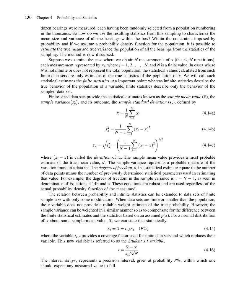
Finite-sized data sets provide the statistical estimates known as the sample mean value (x), the
sample variance s
2
x
À Á
, and its outcome, the sample standard deviation (s x ), defined by
x ¼
1
N
X N
i¼1
x i
ð4:14aÞ
s
2
x ¼
1
N À 1
X N
i¼1
x i À x
ð
Þ
2
ð4:14bÞ
s x ¼
ffiffiffiffi
s 2
x
q
¼
1
N À 1
X N
i¼1
x i À x
ð
Þ
2
! 1=2
ð4:14cÞ
where x i À x
ð
Þ is called the deviation of x i . The sample mean value provides a most probable
estimate of the true mean value, x
0 . The sample variance represents a probable measure of the
variation found in a data set. The degrees of freedom, n, in a statistical estimate equate to the number
of data points minus the number of previously determined statistical parameters used in estimating
that value. For example, the degrees of freedom in the sample variance is n ¼ N À 1, as seen in
denominator of Equations 4.14b and c. These equations are robust and are used regardless of the
actual probability density function of the measurand.
The relation between probability and infinite statistics can be extended to data sets of finite
sample size with only some modification. When data sets are finite or smaller than the population,
the z variable does not provide a reliable weight estimate of the true probability. However, the
sample variance can be weighted in a similar manner so as to compensate for the difference between
the finite statistical estimates and the statistics based on an assumed p(x). For a normal distribution
of x about some sample mean value, x, we can state that statistically
x i ¼ x Æ t n;P s x ðP%Þ
ð 4:15Þ
where the variable t n,P provides a coverage factor used for finite data sets and which replaces the z
variable. This new variable is referred to as the Student’s t variable,
t ¼
x À x
0
s x =
ffiffiffiffi
N
p
ð4:16Þ
The interval Æt n;P s x represents a precision interval, given at probability P%, within which one
should expect any measured value to fall.
130 Chapter 4 Probability and Statistics
14:7:41 Page 130
dozen bearings were measured, each having been randomly selected from a population numbering
in the thousands. So how do we use the resulting statistics from this sampling to characterize the
mean size and variance of all the bearings within the box? Within the constraints imposed by
probability and if we assume a probability density function for the population, it is possible to
estimate the true mean and true variance the population of all the bearings from the statistics of the
sampling. The method is now discussed.
Suppose we examine the case where we obtain N measurements of x (that is, N repetitions),
each measurement represented by x i , where i ¼ 1, 2, . . . , N, and N is a finite value. In cases where
N is not infinite or does not represent the total population, the statistical values calculated from such
finite data sets are only estimates of the true statistics of the population of x. We will call such
statistical estimates the finite statistics. An important point: whereas infinite statistics describe the
true behavior of the population of a variable, finite statistics describe only the behavior of the
sampled data set.
Finite-sized data sets provide the statistical estimates known as the sample mean value (x), the
sample variance s
2
x
À Á
, and its outcome, the sample standard deviation (s x ), defined by
x ¼
1
N
X N
i¼1
x i
ð4:14aÞ
s
2
x ¼
1
N À 1
X N
i¼1
x i À x
ð
Þ
2
ð4:14bÞ
s x ¼
ffiffiffiffi
s 2
x
q
¼
1
N À 1
X N
i¼1
x i À x
ð
Þ
2
! 1=2
ð4:14cÞ
where x i À x
ð
Þ is called the deviation of x i . The sample mean value provides a most probable
estimate of the true mean value, x
0 . The sample variance represents a probable measure of the
variation found in a data set. The degrees of freedom, n, in a statistical estimate equate to the number
of data points minus the number of previously determined statistical parameters used in estimating
that value. For example, the degrees of freedom in the sample variance is n ¼ N À 1, as seen in
denominator of Equations 4.14b and c. These equations are robust and are used regardless of the
actual probability density function of the measurand.
The relation between probability and infinite statistics can be extended to data sets of finite
sample size with only some modification. When data sets are finite or smaller than the population,
the z variable does not provide a reliable weight estimate of the true probability. However, the
sample variance can be weighted in a similar manner so as to compensate for the difference between
the finite statistical estimates and the statistics based on an assumed p(x). For a normal distribution
of x about some sample mean value, x, we can state that statistically
x i ¼ x Æ t n;P s x ðP%Þ
ð 4:15Þ
where the variable t n,P provides a coverage factor used for finite data sets and which replaces the z
variable. This new variable is referred to as the Student’s t variable,
t ¼
x À x
0
s x =
ffiffiffiffi
N
p
ð4:16Þ
The interval Æt n;P s x represents a precision interval, given at probability P%, within which one
should expect any measured value to fall.
130 Chapter 4 Probability and Statistics