

E1C03 09/14/2010
15:24:53 Page 96
system. Examples of second-order instruments include accelerometers and pressure transducers
(including microphones and loudspeakers).
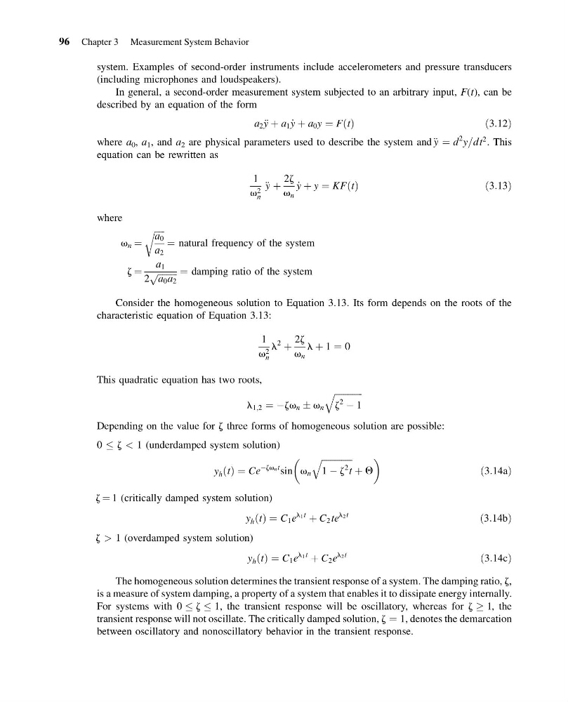
In general, a second-order measurement system subjected to an arbitrary input, F(t), can be
described by an equation of the form
a 2 y € þ a 1 _
y þ a 0 y ¼ F t
ð Þ
ð3:12Þ
where a 0 , a 1 , and a 2 are physical parameters used to describe the system and € y ¼ d
2
y=dt
2 . This
equation can be rewritten as
1
v 2
n
€ y þ
2z
v n
_
y þ y ¼ KF t
ð Þ
ð3:13Þ
where
v n ¼
ffiffiffiffi ffi
a 0
a 2
r
¼ natural frequency of the system
z ¼
a 1
2
ffiffiffiffiffiffiffiffiffi
a 0 a 2
p
¼ damping ratio of the system
Consider the homogeneous solution to Equation 3.13. Its form depends on the roots of the
characteristic equation of Equation 3.13:
1
v 2
n
l
2
þ
2z
v n
l þ 1 ¼ 0
This quadratic equation has two roots,
l 1;2 ¼ Àzv n Æ v n
ffiffiffiffiffiffiffiffiffiffiffiffi ffi
z
2
À 1
q
Depending on the value for z three forms of homogeneous solution are possible:
0 z < 1 (underdamped system solution)
y h ðtÞ ¼ Ce
Àzv n t sin v n
ffiffiffiffiffiffiffiffiffiffiffiffiffiffi
1 À z
2
t
q
þ Q
ð3:14aÞ
z ¼ 1 (critically damped system solution)
y h t
ð Þ ¼ C 1 e
l 1 t
þ C 2 te
l 2 t
ð3:14bÞ
z > 1 (overdamped system solution)
y h ðtÞ ¼ C 1 e
l 1 t
þ C 2 e
l 2 t
ð3:14cÞ
The homogeneous solution determines the transient response of a system. The damping ratio, z,
is a measure of system damping, a property of a system that enables it to dissipate energy internally.
For systems with 0 z 1, the transient response will be oscillatory, whereas for z ! 1, the
transient response will not oscillate. The critically damped solution, z ¼ 1, denotes the demarcation
between oscillatory and nonoscillatory behavior in the transient response.
96 Chapter 3 Measurement System Behavior
15:24:53 Page 96
system. Examples of second-order instruments include accelerometers and pressure transducers
(including microphones and loudspeakers).
In general, a second-order measurement system subjected to an arbitrary input, F(t), can be
described by an equation of the form
a 2 y € þ a 1 _
y þ a 0 y ¼ F t
ð Þ
ð3:12Þ
where a 0 , a 1 , and a 2 are physical parameters used to describe the system and € y ¼ d
2
y=dt
2 . This
equation can be rewritten as
1
v 2
n
€ y þ
2z
v n
_
y þ y ¼ KF t
ð Þ
ð3:13Þ
where
v n ¼
ffiffiffiffi ffi
a 0
a 2
r
¼ natural frequency of the system
z ¼
a 1
2
ffiffiffiffiffiffiffiffiffi
a 0 a 2
p
¼ damping ratio of the system
Consider the homogeneous solution to Equation 3.13. Its form depends on the roots of the
characteristic equation of Equation 3.13:
1
v 2
n
l
2
þ
2z
v n
l þ 1 ¼ 0
This quadratic equation has two roots,
l 1;2 ¼ Àzv n Æ v n
ffiffiffiffiffiffiffiffiffiffiffiffi ffi
z
2
À 1
q
Depending on the value for z three forms of homogeneous solution are possible:
0 z < 1 (underdamped system solution)
y h ðtÞ ¼ Ce
Àzv n t sin v n
ffiffiffiffiffiffiffiffiffiffiffiffiffiffi
1 À z
2
t
q
þ Q
ð3:14aÞ
z ¼ 1 (critically damped system solution)
y h t
ð Þ ¼ C 1 e
l 1 t
þ C 2 te
l 2 t
ð3:14bÞ
z > 1 (overdamped system solution)
y h ðtÞ ¼ C 1 e
l 1 t
þ C 2 e
l 2 t
ð3:14cÞ
The homogeneous solution determines the transient response of a system. The damping ratio, z,
is a measure of system damping, a property of a system that enables it to dissipate energy internally.
For systems with 0 z 1, the transient response will be oscillatory, whereas for z ! 1, the
transient response will not oscillate. The critically damped solution, z ¼ 1, denotes the demarcation
between oscillatory and nonoscillatory behavior in the transient response.
96 Chapter 3 Measurement System Behavior