G.3 Hamilton’s Equations
673
K = H =
f 2 (P )
2m
(cos
2 Q + sin
2 Q) =
f 2 (P )
2m
,
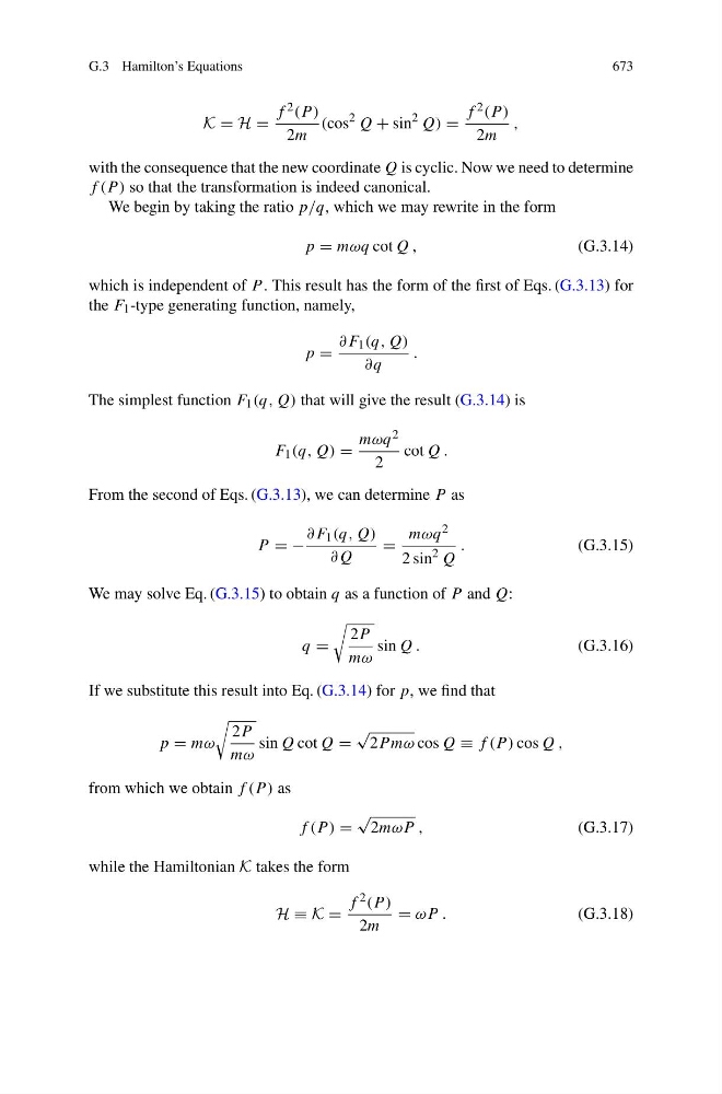
with the consequence that the new coordinate Q is cyclic. Now we need to determine
f (P ) so that the transformation is indeed canonical.
We begin by taking the ratio p/q, which we may rewrite in the form
p = mωq cot Q ,
(G.3.14)
which is independent of P . This result has the form of the first of Eqs. (G.3.13) for
the F 1 -type generating function, namely,
p =
∂F 1 (q, Q)
∂q
.
The simplest function F 1 (q, Q) that will give the result (G.3.14) is
F 1 (q, Q) =
mωq 2
2
cot Q .
From the second of Eqs. (G.3.13), we can determine P as
P = −
∂F 1 (q, Q)
∂Q
=
mωq 2
2 sin
2 Q
.
(G.3.15)
We may solve Eq. (G.3.15) to obtain q as a function of P and Q:
q =
2P
mω
sin Q .
(G.3.16)
If we substitute this result into Eq. (G.3.14) for p, we find that
p = mω
2P
mω
sin Q cot Q =
√
2P mω cos Q ≡ f (P ) cos Q ,
from which we obtain f (P ) as
f (P ) =
√
2mωP ,
(G.3.17)
while the Hamiltonian K takes the form
H ≡ K =
f 2 (P )
2m
= ωP .
(G.3.18)