

646
F Review of Solid State Concepts
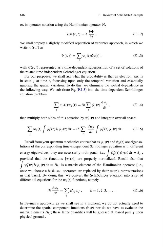
or, in operator notation using the Hamiltonian operator H,
H(r, t) = ¯
h
∂∂
∂t
.
(F.1.2)
We shall employ a slightly modified separation of variables approach, in which we
write (r, t) as
(r, t) =
j
w j (t)ψ j (r) ,
(F.1.3)
with (r, t) represented as a time-dependent superposition of a set of solutions of
the related time-independent Schrödinger equation.
For our purposes, we shall ask what the probability is that an electron, say, is
in state j at time t, focussing upon only the temporal variation and essentially
ignoring the spatial variation. To do this, we eliminate the spatial dependence in
the following way. We substitute Eq. (F.1.3) into the time-dependent Schrödinger
equation to obtain
j
w j (t)ψ j (r) = i ¯
h
j
ψ j (r)
dw j
dt
,
(F.1.4)
then multiply both sides of this equation by ψ ∗
k (r) and integrate over all space:
j
w j (t)
ψ
∗
k (r)Hψ j (r) dr = i ¯
h
j
dw j
dt
ψ
∗
k (r)ψ j (r) dr .
(F.1.5)
Recall from your quantum mechanics course that as ψ j (r) and ψ k (r) are eigensolutions of the corresponding time-independent Schrödinger equation with different
energy eigenvalues, they are necessarily orthogonal, i.e.,
ψ
∗
k (r)ψ j (r) dr = δ jk ,
provided that the functions {ψ i (r)} are properly normalized. Recall also that
ψ
∗
k (r)Hψ j (r) dr ≡ H kj is a matrix element of the Hamiltonian operator [i.e.,
once we choose a basis set, operators are replaced by their matrix representations
in that basis]. By doing this, we convert the Schrödinger equation into a set of
differential equations for the w k (t) functions, namely,
i ¯
h
dw k
dt
=
j
H kj w j ,
k = 1, 2, 3, . . . .
(F.1.6)
In Feyman’s approach, as we shall see in a moment, we do not actually need to
determine the spatial component functions ψ i (r) nor do we have to evaluate the
matrix elements H kj ; these latter quantities will be guessed at, based purely upon
physical grounds.