626
C Stirling Approximations
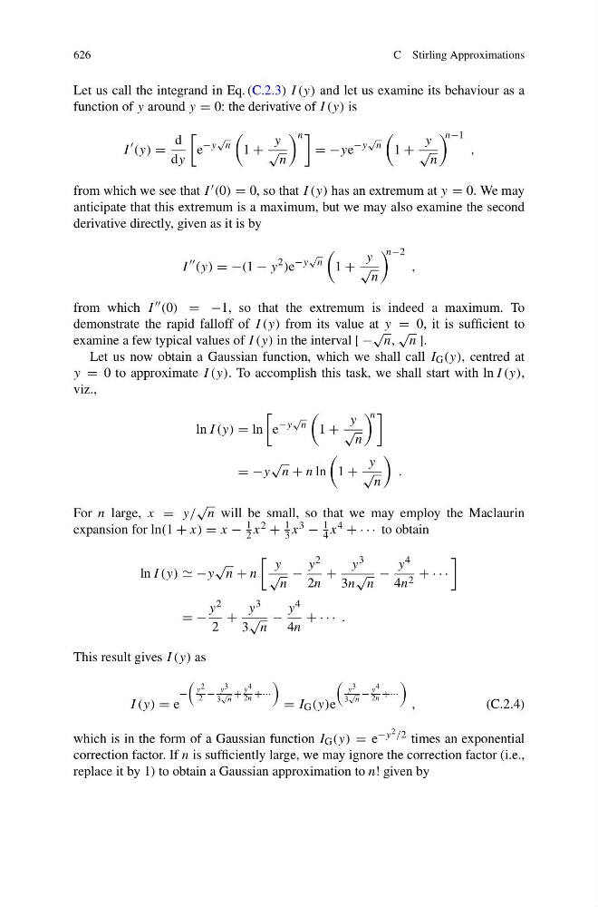
Let us call the integrand in Eq. (C.2.3) I (y) and let us examine its behaviour as a
function of y around y = 0: the derivative of I (y) is
I
(y) =
d
dy
e
−y
√
n
1 +
y
√
n
n
= −ye
−y
√
n
1 +
y
√
n
n−1
,
from which we see that I (0) = 0, so that I (y) has an extremum at y = 0. We may
anticipate that this extremum is a maximum, but we may also examine the second
derivative directly, given as it is by
I
(y) = −(1 − y
2 )e
−y
√
n
1 +
y
√
n
n−2
,
from which I (0) = −1, so that the extremum is indeed a maximum. To
demonstrate the rapid falloff of I (y) from its value at y = 0, it is sufficient to
examine a few typical values of I (y) in the interval [ −
√
n,
√
n ].
Let us now obtain a Gaussian function, which we shall call I G (y), centred at
y = 0 to approximate I (y). To accomplish this task, we shall start with ln I (y),
viz.,
ln I (y) = ln
e
−y
√
n
1 +
y
√
n
n
= −y
√
n + n ln
1 +
y
√
n
.
For n large, x = y/
√
n will be small, so that we may employ the Maclaurin
expansion for ln(1 + x) = x −
1
2 x 2 +
1
3 x 3 −
1
4 x 4 + · · · to obtain
ln I (y) −y
√
n + n
y
√
n
−
y 2
2n
+
y 3
3n
√
n
−
y 4
4n 2 + · · ·
= −
y 2
2
+
y 3
3
√
n
−
y 4
4n
+ · · · .
This result gives I (y) as
I (y) = e
−
y 2
2 −
y 3
3
√
n
+
y 4
2n +···
= I G (y)e
y 3
3
√
n
−
y 4
2n +···
,
(C.2.4)
which is in the form of a Gaussian function I G (y) = e −y 2 /2 times an exponential
correction factor. If n is sufficiently large, we may ignore the correction factor (i.e.,
replace it by 1) to obtain a Gaussian approximation to n! given by