

614
B Review of Traditional Calculus
B.2 Legendre Transforms
In the simplest (i.e., one-dimensional) case, the Legendre transform provides the
procedure whereby the relation y = y(x), which we may represent as a curve in the
Cartesian xy-plane with the tangent lines to it at points (x, y) having slopes given
by the derivative y (x), can be interpreted as the envelope of a set of tangent lines.
Elimination of the variable x between y(x) and y (x) gives y as a function of y .
We may express the tangent line t (x) passing through the point (x, y) on the
curve generated by y = y(x) as
t (x) = y
x + t i ,
(B.2.1a)
with y its slope and t i its y-intercept. By writing the slope y explicitly in the form
y
=
y − t i
x − 0
,
(B.2.1b)
we may generate the set of y-intercepts associated with the tangent lines to the curve
y = y(x) from the expression
t i (x) = y − y
x .
(B.2.2a)
We shall refer to this expression for t i as the Legendre transform of y. This set of
tangent lines is equivalent to the curve y = y(x), as we shall now illustrate explicitly
with a very simple example.
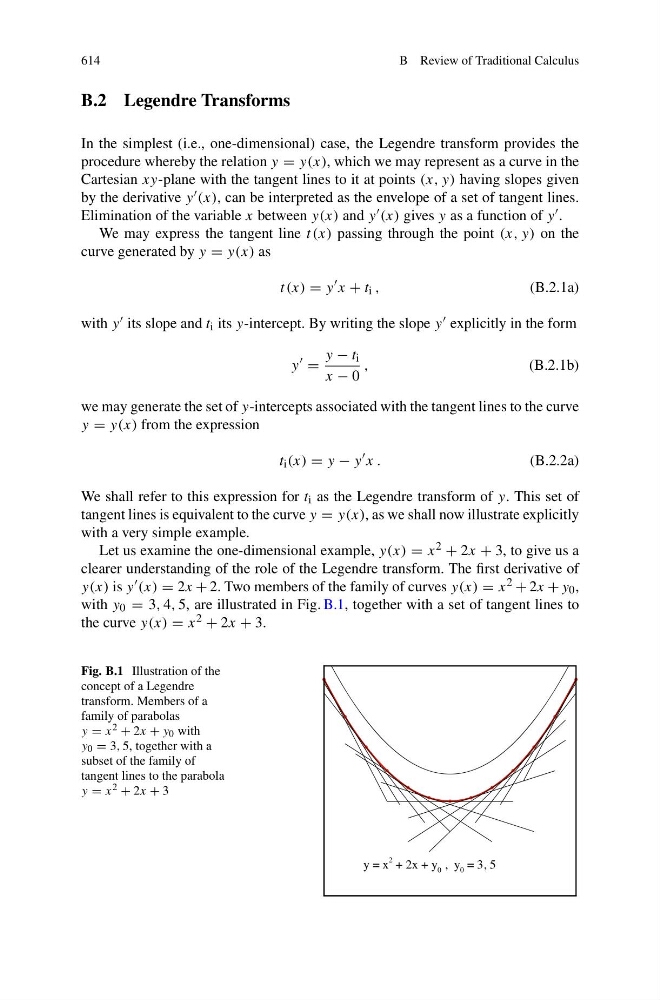
Let us examine the one-dimensional example, y(x) = x 2 + 2x + 3, to give us a
clearer understanding of the role of the Legendre transform. The first derivative of
y(x) is y (x) = 2x + 2. Two members of the family of curves y(x) = x 2 + 2x + y 0 ,
with y 0 = 3, 4, 5, are illustrated in Fig. B.1, together with a set of tangent lines to
the curve y(x) = x 2 + 2x + 3.
Fig. B.1 Illustration of the
concept of a Legendre
transform. Members of a
family of parabolas
y = x 2 + 2x + y 0 with
y 0 = 3, 5, together with a
subset of the family of
tangent lines to the parabola
y = x 2 + 2x + 3