

10.4 Fermi–Dirac Statistics
541
U N
ce k B T =
N ce k B
2 T 2
F
.
(10.4.27)
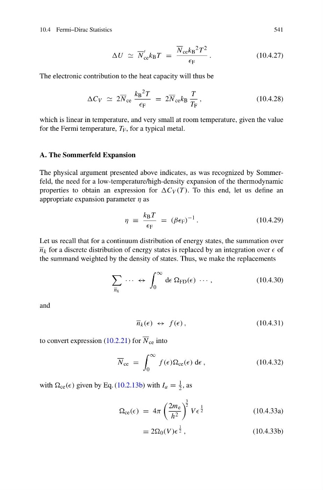
The electronic contribution to the heat capacity will thus be
C V 2N ce
k B
2 T
F
= 2N ce k B
T
T F
,
(10.4.28)
which is linear in temperature, and very small at room temperature, given the value
for the Fermi temperature, T F , for a typical metal.
A. The Sommerfeld Expansion
The physical argument presented above indicates, as was recognized by Sommerfeld, the need for a low-temperature/high-density expansion of the thermodynamic
properties to obtain an expression for C V (T ). To this end, let us define an
appropriate expansion parameter η as
η ≡
k B T
F
= (ββ F )
−1 .
(10.4.29)
Let us recall that for a continuum distribution of energy states, the summation over
n k for a discrete distribution of energy states is replaced by an integration over of
the summand weighted by the density of states. Thus, we make the replacements
n k
· · · ↔
∞
0
d FD (() · · · ,
(10.4.30)
and
n k (() ↔ f (() ,
(10.4.31)
to convert expression (10.2.21) for N ce into
N ce =
∞
0
f (()) ce (() d ,
(10.4.32)
with ce (() given by Eq. (10.2.13b) with I a =
1
2 , as
ce (() = 4π
2m e
h 2
3
2
V V
1
2
(10.4.33a)
≡ 2 0 (V ))
1
2 ,
(10.4.33b)
541
U N
ce k B T =
N ce k B
2 T 2
F
.
(10.4.27)
The electronic contribution to the heat capacity will thus be
C V 2N ce
k B
2 T
F
= 2N ce k B
T
T F
,
(10.4.28)
which is linear in temperature, and very small at room temperature, given the value
for the Fermi temperature, T F , for a typical metal.
A. The Sommerfeld Expansion
The physical argument presented above indicates, as was recognized by Sommerfeld, the need for a low-temperature/high-density expansion of the thermodynamic
properties to obtain an expression for C V (T ). To this end, let us define an
appropriate expansion parameter η as
η ≡
k B T
F
= (ββ F )
−1 .
(10.4.29)
Let us recall that for a continuum distribution of energy states, the summation over
n k for a discrete distribution of energy states is replaced by an integration over of
the summand weighted by the density of states. Thus, we make the replacements
n k
· · · ↔
∞
0
d FD (() · · · ,
(10.4.30)
and
n k (() ↔ f (() ,
(10.4.31)
to convert expression (10.2.21) for N ce into
N ce =
∞
0
f (()) ce (() d ,
(10.4.32)
with ce (() given by Eq. (10.2.13b) with I a =
1
2 , as
ce (() = 4π
2m e
h 2
3
2
V V
1
2
(10.4.33a)
≡ 2 0 (V ))
1
2 ,
(10.4.33b)