

10.1 Setting the Stage
513
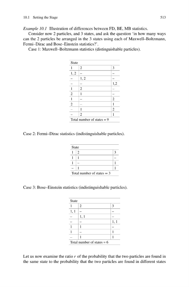
Example 10.1 Illustration of differences between FD, BE, MB statistics.
Consider now 2 particles, and 3 states, and ask the question ‘in how many ways
can the 2 particles be arranged in the 3 states using each of Maxwell–Boltzmann,
Fermi–Dirac and Bose–Einstein statistics?’.
Case 1: Maxwell–Boltzmann statistics (distinguishable particles).
State
1
2
3
1, 2 –
–
–
1, 2
–
–
–
1,2
1
2
–
2
1
–
1
–
2
2
–
1
–
1
2
–
2
1
Total number of states = 9
Case 2: Fermi–Dirac statistics (indistinguishable particles).
State
1 2
3
1 1
–
1 –
1
– 1
1
Total number of states = 3
Case 3: Bose–Einstein statistics (indistinguishable particles).
State
1
2
3
1, 1 –
–
–
1, 1
–
–
–
1, 1
1
1
–
1
–
1
–
1
1
Total number of states = 6
Let us now examine the ratio r of the probability that the two particles are found in
the same state to the probability that the two particles are found in different states
513
Example 10.1 Illustration of differences between FD, BE, MB statistics.
Consider now 2 particles, and 3 states, and ask the question ‘in how many ways
can the 2 particles be arranged in the 3 states using each of Maxwell–Boltzmann,
Fermi–Dirac and Bose–Einstein statistics?’.
Case 1: Maxwell–Boltzmann statistics (distinguishable particles).
State
1
2
3
1, 2 –
–
–
1, 2
–
–
–
1,2
1
2
–
2
1
–
1
–
2
2
–
1
–
1
2
–
2
1
Total number of states = 9
Case 2: Fermi–Dirac statistics (indistinguishable particles).
State
1 2
3
1 1
–
1 –
1
– 1
1
Total number of states = 3
Case 3: Bose–Einstein statistics (indistinguishable particles).
State
1
2
3
1, 1 –
–
–
1, 1
–
–
–
1, 1
1
1
–
1
–
1
–
1
1
Total number of states = 6
Let us now examine the ratio r of the probability that the two particles are found in
the same state to the probability that the two particles are found in different states