

384
7 Classical Statistical Mechanics
the net change for the full phase-space volume element, and in step 3 we shall equate
the result of step 2 with the change in the distribution function f (N ) for that phase
volume.
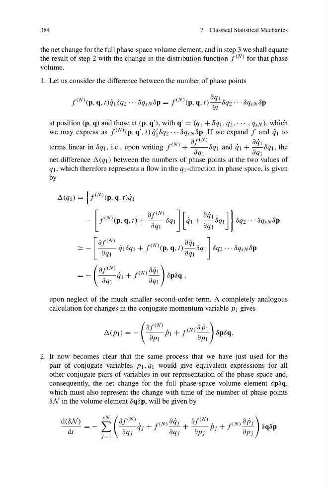
1. Let us consider the difference between the number of phase points
f
(N ) (p, q, t) ˙
q 1 δq 2 · · · δq sN δp = f
(N ) (p, q, t)
∂q 1
∂t
δq 2 · · · δq sN δp
at position (p, q) and those at (p, q ), with q = (q 1 + δq 1 , q 2 , · · · , q sN ), which
we may express as f (N ) (p, q , t) ˙
q
1 δq 2 · · · δq sN δp. If we expand f and ˙
q 1 to
terms linear in δq 1 , i.e., upon writing f
(N )
+
∂f (N )
∂q 1
δq 1 and ˙
q 1 +
∂ ˙
q 1
∂q 1
δq 1 , the
net difference (q 1 ) between the numbers of phase points at the two values of
q 1 , which therefore represents a flow in the q 1 -direction in phase space, is given
by
(q 1 ) =
f
(N ) (p, q, t) ˙
q 1
−
f
(N ) (p, q, t) +
∂f (N )
∂q 1
δq 1
˙
q 1 +
∂ ˙
q 1
∂q 1
δq 1
δq 2 · · · δq sN δp
−
∂f (N )
∂q 1
˙
q 1 δq 1 + f
(N ) (p, q, t)
∂ ˙
q 1
∂q 1
δq 1
δq 2 · · · δq sN δp
= −
∂f (N )
∂q 1
˙
q 1 + f
(N ) ∂ ˙
q 1
∂q 1
δpδq ,
upon neglect of the much smaller second-order term. A completely analogous
calculation for changes in the conjugate momentum variable p 1 gives
(p 1 ) = −
∂f (N )
∂p 1
˙
p 1 + f
(N ) ∂ ˙
p 1
∂p 1
δpδq.
2. It now becomes clear that the same process that we have just used for the
pair of conjugate variables p 1 , q 1 would give equivalent expressions for all
other conjugate pairs of variables in our representation of the phase space and,
consequently, the net change for the full phase-space volume element δpδq,
which must also represent the change with time of the number of phase points
δN in the volume element δqδp, will be given by
d(δN )
dt
= −
sN
j =1
∂f (N )
∂q j
˙
q j + f
(N ) ∂ ˙
q j
∂q j
+
∂f (N )
∂p j
˙
p j + f
(N ) ∂ ˙
p j
∂p j
δqδp
7 Classical Statistical Mechanics
the net change for the full phase-space volume element, and in step 3 we shall equate
the result of step 2 with the change in the distribution function f (N ) for that phase
volume.
1. Let us consider the difference between the number of phase points
f
(N ) (p, q, t) ˙
q 1 δq 2 · · · δq sN δp = f
(N ) (p, q, t)
∂q 1
∂t
δq 2 · · · δq sN δp
at position (p, q) and those at (p, q ), with q = (q 1 + δq 1 , q 2 , · · · , q sN ), which
we may express as f (N ) (p, q , t) ˙
q
1 δq 2 · · · δq sN δp. If we expand f and ˙
q 1 to
terms linear in δq 1 , i.e., upon writing f
(N )
+
∂f (N )
∂q 1
δq 1 and ˙
q 1 +
∂ ˙
q 1
∂q 1
δq 1 , the
net difference (q 1 ) between the numbers of phase points at the two values of
q 1 , which therefore represents a flow in the q 1 -direction in phase space, is given
by
(q 1 ) =
f
(N ) (p, q, t) ˙
q 1
−
f
(N ) (p, q, t) +
∂f (N )
∂q 1
δq 1
˙
q 1 +
∂ ˙
q 1
∂q 1
δq 1
δq 2 · · · δq sN δp
−
∂f (N )
∂q 1
˙
q 1 δq 1 + f
(N ) (p, q, t)
∂ ˙
q 1
∂q 1
δq 1
δq 2 · · · δq sN δp
= −
∂f (N )
∂q 1
˙
q 1 + f
(N ) ∂ ˙
q 1
∂q 1
δpδq ,
upon neglect of the much smaller second-order term. A completely analogous
calculation for changes in the conjugate momentum variable p 1 gives
(p 1 ) = −
∂f (N )
∂p 1
˙
p 1 + f
(N ) ∂ ˙
p 1
∂p 1
δpδq.
2. It now becomes clear that the same process that we have just used for the
pair of conjugate variables p 1 , q 1 would give equivalent expressions for all
other conjugate pairs of variables in our representation of the phase space and,
consequently, the net change for the full phase-space volume element δpδq,
which must also represent the change with time of the number of phase points
δN in the volume element δqδp, will be given by
d(δN )
dt
= −
sN
j =1
∂f (N )
∂q j
˙
q j + f
(N ) ∂ ˙
q j
∂q j
+
∂f (N )
∂p j
˙
p j + f
(N ) ∂ ˙
p j
∂p j
δqδp