

364
7 Classical Statistical Mechanics
for a container of infinite volume. However, for a container of finite volume, such
that the first term in Eq. (7.1.9) cannot be said to vanish, then Eq. (7.1.11a) will fail.
Such a failure is averted via the introduction of a wall potential W (r) that goes to
infinity at the confining vessel boundaries, and has a range that is small relative
to the vessel size. Moreover, this example illustrates the importance of taking into
consideration the presence and role, albeit implicit, of system (container) walls.
The role played by wall potential(s) in the classical equipartition principle has
been examined by Mello and Rodríguez [2] for a single particle confined to a 1dimensional potential well. As such an example illustrates the importance and role
of confinement, and as generalization to simple three-dimensional geometries is
relatively straightforward, we shall follow the same approach here.
The Hamiltonian for a single particle located within the interval a ≤ x ≤ b and
possessing kinetic energy p 2 /(2m), potential energy V tot (x) is given by
H 1 =
p 2
2m
+ V tot (x) .
(7.1.12)
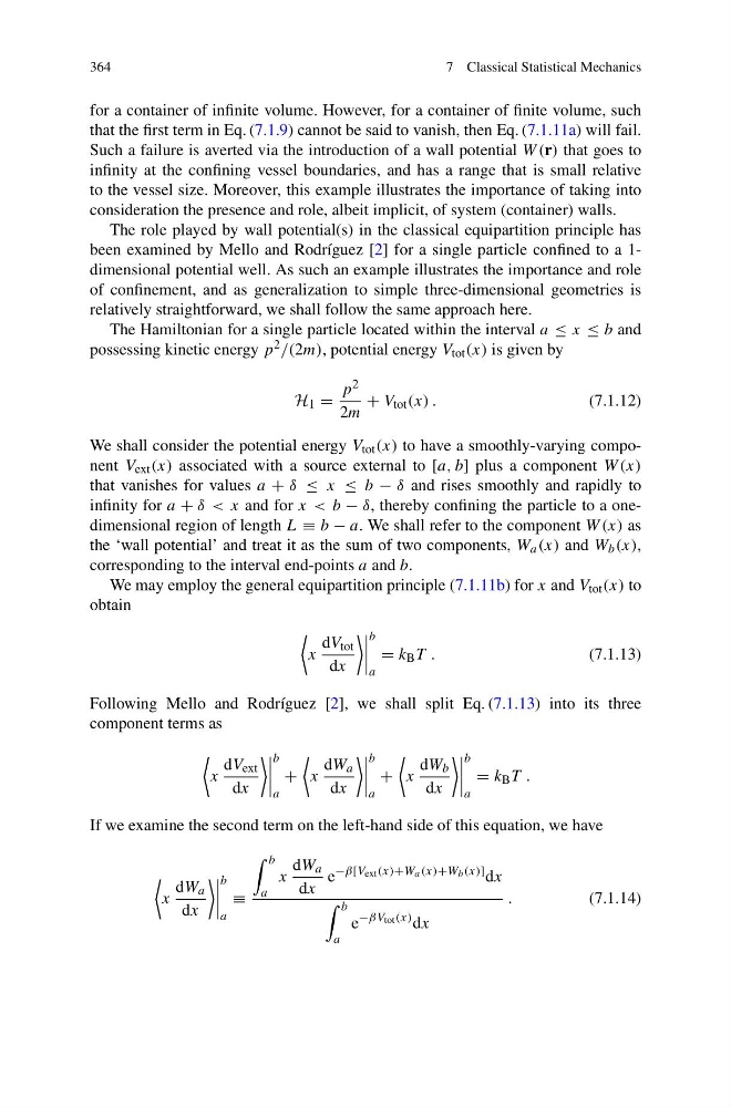
We shall consider the potential energy V tot (x) to have a smoothly-varying component V ext (x) associated with a source external to [a, b] plus a component W (x)
that vanishes for values a + δ ≤ x ≤ b − δ and rises smoothly and rapidly to
infinity for a + δ < x and for x < b − δ, thereby confining the particle to a onedimensional region of length L ≡ b − a. We shall refer to the component W (x) as
the ‘wall potential’ and treat it as the sum of two components, W a (x) and W b (x),
corresponding to the interval end-points a and b.
We may employ the general equipartition principle (7.1.11b) for x and V tot (x) to
obtain
x
dV tot
dx
b
a
= k B T .
(7.1.13)
Following Mello and Rodríguez [2], we shall split Eq. (7.1.13) into its three
component terms as
x
dV ext
dx
b
a
+
x
dW a
dx
b
a
+
x
dW b
dx
b
a
= k B T .
If we examine the second term on the left-hand side of this equation, we have
x
dW a
dx
b
a
≡
b
a
x
dW a
dx
e
−β[V ext (x)+W a (x)+W b (x)] dx
b
a
e
−βV tot (x) dx
.
(7.1.14)
7 Classical Statistical Mechanics
for a container of infinite volume. However, for a container of finite volume, such
that the first term in Eq. (7.1.9) cannot be said to vanish, then Eq. (7.1.11a) will fail.
Such a failure is averted via the introduction of a wall potential W (r) that goes to
infinity at the confining vessel boundaries, and has a range that is small relative
to the vessel size. Moreover, this example illustrates the importance of taking into
consideration the presence and role, albeit implicit, of system (container) walls.
The role played by wall potential(s) in the classical equipartition principle has
been examined by Mello and Rodríguez [2] for a single particle confined to a 1dimensional potential well. As such an example illustrates the importance and role
of confinement, and as generalization to simple three-dimensional geometries is
relatively straightforward, we shall follow the same approach here.
The Hamiltonian for a single particle located within the interval a ≤ x ≤ b and
possessing kinetic energy p 2 /(2m), potential energy V tot (x) is given by
H 1 =
p 2
2m
+ V tot (x) .
(7.1.12)
We shall consider the potential energy V tot (x) to have a smoothly-varying component V ext (x) associated with a source external to [a, b] plus a component W (x)
that vanishes for values a + δ ≤ x ≤ b − δ and rises smoothly and rapidly to
infinity for a + δ < x and for x < b − δ, thereby confining the particle to a onedimensional region of length L ≡ b − a. We shall refer to the component W (x) as
the ‘wall potential’ and treat it as the sum of two components, W a (x) and W b (x),
corresponding to the interval end-points a and b.
We may employ the general equipartition principle (7.1.11b) for x and V tot (x) to
obtain
x
dV tot
dx
b
a
= k B T .
(7.1.13)
Following Mello and Rodríguez [2], we shall split Eq. (7.1.13) into its three
component terms as
x
dV ext
dx
b
a
+
x
dW a
dx
b
a
+
x
dW b
dx
b
a
= k B T .
If we examine the second term on the left-hand side of this equation, we have
x
dW a
dx
b
a
≡
b
a
x
dW a
dx
e
−β[V ext (x)+W a (x)+W b (x)] dx
b
a
e
−βV tot (x) dx
.
(7.1.14)