

302
14 Amplitude Factorization and Feynman Diagrams
(a)
(b)
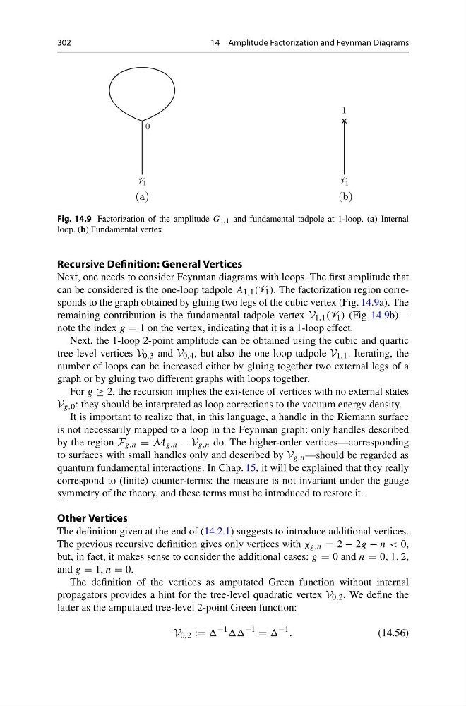
Fig. 14.9 Factorization of the amplitude G 1,1 and fundamental tadpole at 1-loop. (a) Internal
loop. (b) Fundamental vertex
Recursive Definition: General Vertices
Next, one needs to consider Feynman diagrams with loops. The first amplitude that
can be considered is the one-loop tadpole A 1,1 (V 1 ). The factorization region corresponds to the graph obtained by gluing two legs of the cubic vertex (Fig. 14.9a). The
remaining contribution is the fundamental tadpole vertex V 1,1 (V 1 ) (Fig. 14.9b)—
note the index g = 1 on the vertex, indicating that it is a 1-loop effect.
Next, the 1-loop 2-point amplitude can be obtained using the cubic and quartic
tree-level vertices V 0,3 and V 0,4 , but also the one-loop tadpole V 1,1 . Iterating, the
number of loops can be increased either by gluing together two external legs of a
graph or by gluing two different graphs with loops together.
For g ≥ 2, the recursion implies the existence of vertices with no external states
V g,0 : they should be interpreted as loop corrections to the vacuum energy density.
It is important to realize that, in this language, a handle in the Riemann surface
is not necessarily mapped to a loop in the Feynman graph: only handles described
by the region F g,n = M g,n − V g,n do. The higher-order vertices—corresponding
to surfaces with small handles only and described by V g,n —should be regarded as
quantum fundamental interactions. In Chap. 15, it will be explained that they really
correspond to (finite) counter-terms: the measure is not invariant under the gauge
symmetry of the theory, and these terms must be introduced to restore it.
Other Vertices
The definition given at the end of (14.2.1) suggests to introduce additional vertices.
The previous recursive definition gives only vertices with χ g,n = 2 − 2g − n < 0,
but, in fact, it makes sense to consider the additional cases: g = 0 and n = 0, 1, 2,
and g = 1, n = 0.
The definition of the vertices as amputated Green function without internal
propagators provides a hint for the tree-level quadratic vertex V 0,2 . We define the
latter as the amputated tree-level 2-point Green function:
V 0,2 :=
−1
−1
=
−1 .
(14.56)
14 Amplitude Factorization and Feynman Diagrams
(a)
(b)
Fig. 14.9 Factorization of the amplitude G 1,1 and fundamental tadpole at 1-loop. (a) Internal
loop. (b) Fundamental vertex
Recursive Definition: General Vertices
Next, one needs to consider Feynman diagrams with loops. The first amplitude that
can be considered is the one-loop tadpole A 1,1 (V 1 ). The factorization region corresponds to the graph obtained by gluing two legs of the cubic vertex (Fig. 14.9a). The
remaining contribution is the fundamental tadpole vertex V 1,1 (V 1 ) (Fig. 14.9b)—
note the index g = 1 on the vertex, indicating that it is a 1-loop effect.
Next, the 1-loop 2-point amplitude can be obtained using the cubic and quartic
tree-level vertices V 0,3 and V 0,4 , but also the one-loop tadpole V 1,1 . Iterating, the
number of loops can be increased either by gluing together two external legs of a
graph or by gluing two different graphs with loops together.
For g ≥ 2, the recursion implies the existence of vertices with no external states
V g,0 : they should be interpreted as loop corrections to the vacuum energy density.
It is important to realize that, in this language, a handle in the Riemann surface
is not necessarily mapped to a loop in the Feynman graph: only handles described
by the region F g,n = M g,n − V g,n do. The higher-order vertices—corresponding
to surfaces with small handles only and described by V g,n —should be regarded as
quantum fundamental interactions. In Chap. 15, it will be explained that they really
correspond to (finite) counter-terms: the measure is not invariant under the gauge
symmetry of the theory, and these terms must be introduced to restore it.
Other Vertices
The definition given at the end of (14.2.1) suggests to introduce additional vertices.
The previous recursive definition gives only vertices with χ g,n = 2 − 2g − n < 0,
but, in fact, it makes sense to consider the additional cases: g = 0 and n = 0, 1, 2,
and g = 1, n = 0.
The definition of the vertices as amputated Green function without internal
propagators provides a hint for the tree-level quadratic vertex V 0,2 . We define the
latter as the amputated tree-level 2-point Green function:
V 0,2 :=
−1
−1
=
−1 .
(14.56)