

12.1 Parametrization of P g,n
253
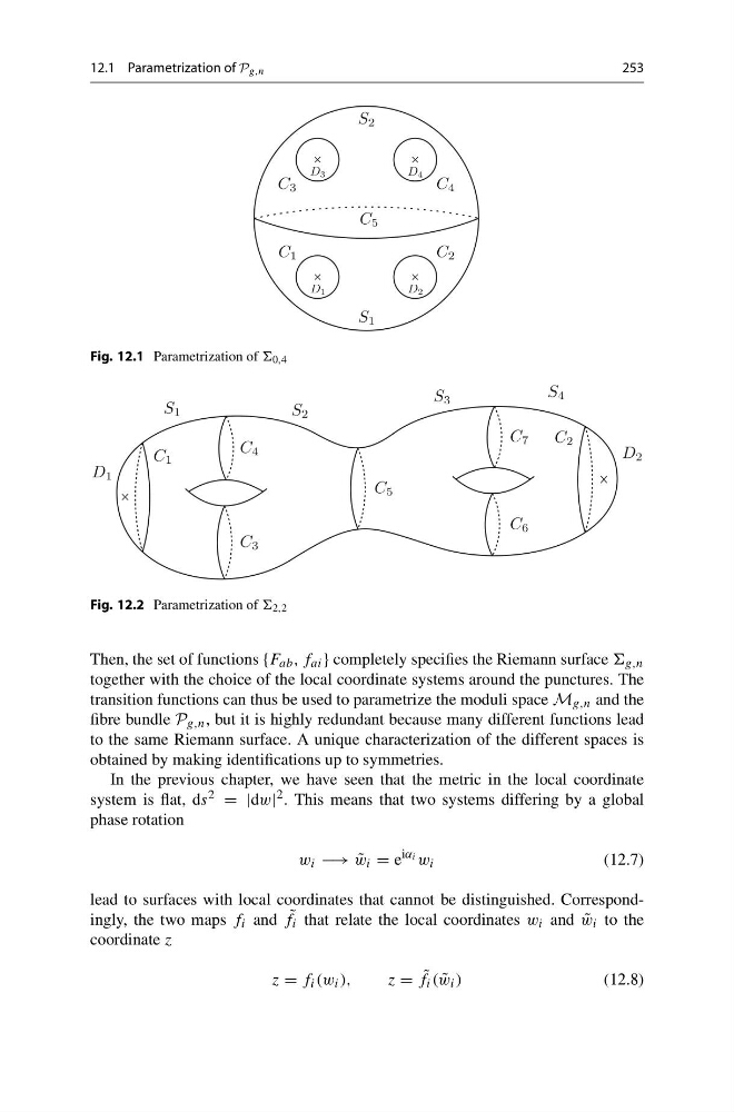
Fig. 12.1 Parametrization of 0,4
Fig. 12.2 Parametrization of 2,2
Then, the set of functions {F ab , f ai } completely specifies the Riemann surface g,n
together with the choice of the local coordinate systems around the punctures. The
transition functions can thus be used to parametrize the moduli space M g,n and the
fibre bundle P g,n , but it is highly redundant because many different functions lead
to the same Riemann surface. A unique characterization of the different spaces is
obtained by making identifications up to symmetries.
In the previous chapter, we have seen that the metric in the local coordinate
system is flat, ds 2 = |dw|
2 . This means that two systems differing by a global
phase rotation
w i −→ ˜
w i = e
iα i w i
(12.7)
lead to surfaces with local coordinates that cannot be distinguished. Correspondingly, the two maps f i and ˜
f i that relate the local coordinates w i and ˜
w i to the
coordinate z
z = f i (w i ),
z = ˜
f i ( ˜
w i )
(12.8)
253
Fig. 12.1 Parametrization of 0,4
Fig. 12.2 Parametrization of 2,2
Then, the set of functions {F ab , f ai } completely specifies the Riemann surface g,n
together with the choice of the local coordinate systems around the punctures. The
transition functions can thus be used to parametrize the moduli space M g,n and the
fibre bundle P g,n , but it is highly redundant because many different functions lead
to the same Riemann surface. A unique characterization of the different spaces is
obtained by making identifications up to symmetries.
In the previous chapter, we have seen that the metric in the local coordinate
system is flat, ds 2 = |dw|
2 . This means that two systems differing by a global
phase rotation
w i −→ ˜
w i = e
iα i w i
(12.7)
lead to surfaces with local coordinates that cannot be distinguished. Correspondingly, the two maps f i and ˜
f i that relate the local coordinates w i and ˜
w i to the
coordinate z
z = f i (w i ),
z = ˜
f i ( ˜
w i )
(12.8)