

144
7 CFT Systems
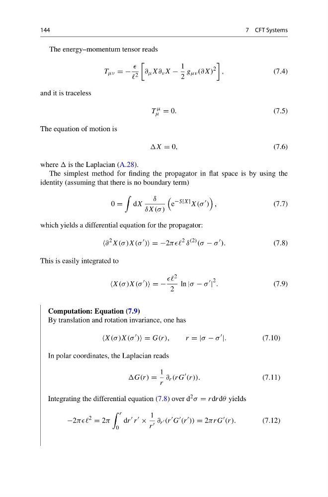
The energy–momentum tensor reads
T μν = −
2
∂ μ X∂ ν X −
1
2
g μν (∂X)
2
,
(7.4)
and it is traceless
T
μ
μ = 0.
(7.5)
The equation of motion is
X = 0,
(7.6)
where is the Laplacian (A.28).
The simplest method for finding the propagator in flat space is by using the
identity (assuming that there is no boundary term)
0 =
dX
δ
δX(σ )
e
−S[X] X(σ
)
,
(7.7)
which yields a differential equation for the propagator:
∂
2 X(σ )X(σ
) = −2πππ
2 δ
(2) (σ − σ
).
(7.8)
This is easily integrated to
X(σ )X(σ
) = −
2
2
ln |σ − σ
|
2 .
(7.9)
Computation: Equation (7.9)
By translation and rotation invariance, one has
X(σ )X(σ
) = G(r),
r = |σ − σ
|.
(7.10)
In polar coordinates, the Laplacian reads
G(r) =
1
r
∂ r (rG
(r)).
(7.11)
Integrating the differential equation (7.8) over d 2 σ = rdrdθ yields
−2πππ
2
= 2π
r
0
dr
r
×
1
r ∂ r (r
G
(r
)) = 2πrG
(r).
(7.12)
7 CFT Systems
The energy–momentum tensor reads
T μν = −
2
∂ μ X∂ ν X −
1
2
g μν (∂X)
2
,
(7.4)
and it is traceless
T
μ
μ = 0.
(7.5)
The equation of motion is
X = 0,
(7.6)
where is the Laplacian (A.28).
The simplest method for finding the propagator in flat space is by using the
identity (assuming that there is no boundary term)
0 =
dX
δ
δX(σ )
e
−S[X] X(σ
)
,
(7.7)
which yields a differential equation for the propagator:
∂
2 X(σ )X(σ
) = −2πππ
2 δ
(2) (σ − σ
).
(7.8)
This is easily integrated to
X(σ )X(σ
) = −
2
2
ln |σ − σ
|
2 .
(7.9)
Computation: Equation (7.9)
By translation and rotation invariance, one has
X(σ )X(σ
) = G(r),
r = |σ − σ
|.
(7.10)
In polar coordinates, the Laplacian reads
G(r) =
1
r
∂ r (rG
(r)).
(7.11)
Integrating the differential equation (7.8) over d 2 σ = rdrdθ yields
−2πππ
2
= 2π
r
0
dr
r
×
1
r ∂ r (r
G
(r
)) = 2πrG
(r).
(7.12)