

6.4 Operator Formalism and Radial Quantization
121
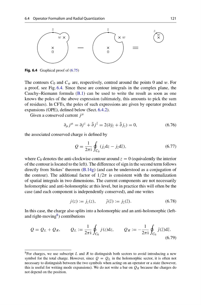
Fig. 6.4 Graphical proof of (6.75)
The contours C 0 and C w are, respectively, centred around the points 0 and w. For
a proof, see Fig. 6.4. Since these are contour integrals in the complex plane, the
Cauchy–Riemann formula (B.1) can be used to write the result as soon as one
knows the poles of the above expression (ultimately, this amounts to pick the sum
of residues). In CFTs, the poles of such expressions are given by operator product
expansions (OPE), defined below (Sect. 6.4.2).
Given a conserved current j μ
∂ μ j
μ
= ∂j
z
+ ¯
∂j
¯
z
= 2(∂j ¯
z + ¯
∂j z ) = 0,
(6.76)
the associated conserved charge is defined by
Q =
1
2π i
C 0
(j z dz − j ¯
z d¯ z),
(6.77)
where C 0 denotes the anti-clockwise contour around z = 0 (equivalently the interior
of the contour is located to the left). The difference of sign in the second term follows
directly from Stokes’ theorem (B.14g) (and can be understood as a conjugation of
the contour). The additional factor of 1/2π is consistent with the normalization
of spatial integrals in two dimensions. The current components are not necessarily
holomorphic and anti-holomorphic at this level, but in practice this will often be the
case (and each component is independently conserved), and one writes
j (z) := j z (z),
¯
j(¯ z) := j ¯
z (¯ z).
(6.78)
In this case, the charge also splits into a holomorphic and an anti-holomorphic (leftand right-moving 8 ) contributions
Q = Q L + Q R ,
Q L :=
1
2π i
C 0
j (z)dz,
Q R := −
1
2π i
C 0
¯
j(¯ z)d¯ z.
(6.79)
8 For charges, we use subscript L and R to distinguish both sectors to avoid introducing a new
symbol for the total charge. However, since Q = Q L in the holomorphic sector, it is often not
necessary to distinguish between the two symbols when acting on an operator or a state (however,
this is useful for writing mode expansions). We do not write a bar on Q R because the charges do
not depend on the position.
121
Fig. 6.4 Graphical proof of (6.75)
The contours C 0 and C w are, respectively, centred around the points 0 and w. For
a proof, see Fig. 6.4. Since these are contour integrals in the complex plane, the
Cauchy–Riemann formula (B.1) can be used to write the result as soon as one
knows the poles of the above expression (ultimately, this amounts to pick the sum
of residues). In CFTs, the poles of such expressions are given by operator product
expansions (OPE), defined below (Sect. 6.4.2).
Given a conserved current j μ
∂ μ j
μ
= ∂j
z
+ ¯
∂j
¯
z
= 2(∂j ¯
z + ¯
∂j z ) = 0,
(6.76)
the associated conserved charge is defined by
Q =
1
2π i
C 0
(j z dz − j ¯
z d¯ z),
(6.77)
where C 0 denotes the anti-clockwise contour around z = 0 (equivalently the interior
of the contour is located to the left). The difference of sign in the second term follows
directly from Stokes’ theorem (B.14g) (and can be understood as a conjugation of
the contour). The additional factor of 1/2π is consistent with the normalization
of spatial integrals in two dimensions. The current components are not necessarily
holomorphic and anti-holomorphic at this level, but in practice this will often be the
case (and each component is independently conserved), and one writes
j (z) := j z (z),
¯
j(¯ z) := j ¯
z (¯ z).
(6.78)
In this case, the charge also splits into a holomorphic and an anti-holomorphic (leftand right-moving 8 ) contributions
Q = Q L + Q R ,
Q L :=
1
2π i
C 0
j (z)dz,
Q R := −
1
2π i
C 0
¯
j(¯ z)d¯ z.
(6.79)
8 For charges, we use subscript L and R to distinguish both sectors to avoid introducing a new
symbol for the total charge. However, since Q = Q L in the holomorphic sector, it is often not
necessary to distinguish between the two symbols when acting on an operator or a state (however,
this is useful for writing mode expansions). We do not write a bar on Q R because the charges do
not depend on the position.