

86
3 Worldsheet Path Integral: Scattering Amplitudes
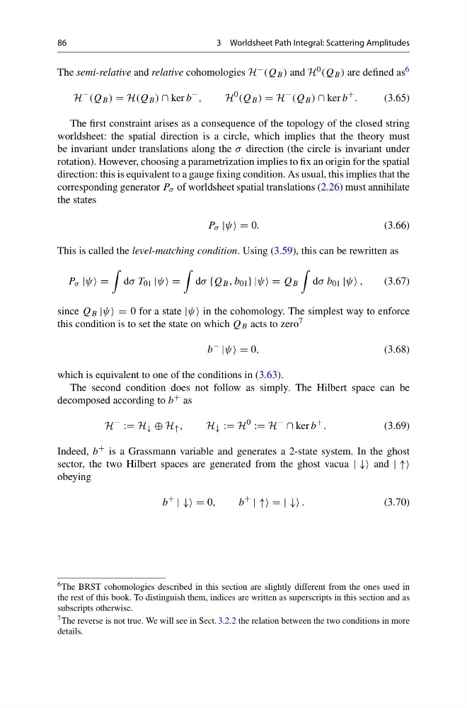
The semi-relative and relative cohomologies H − (Q B ) and H 0 (Q B ) are defined as 6
H
− (Q B ) = H(Q B ) ∩ ker b
− ,
H
0 (Q B ) = H
− (Q B ) ∩ ker b
+ .
(3.65)
The first constraint arises as a consequence of the topology of the closed string
worldsheet: the spatial direction is a circle, which implies that the theory must
be invariant under translations along the σ direction (the circle is invariant under
rotation). However, choosing a parametrization implies to fix an origin for the spatial
direction: this is equivalent to a gauge fixing condition. As usual, this implies that the
corresponding generator P σ of worldsheet spatial translations (2.26) must annihilate
the states
P σ |ψ = 0.
(3.66)
This is called the level-matching condition. Using (3.59), this can be rewritten as
P σ |ψ =
dσ T 01 |ψ =
dσ {Q B , b 01 } |ψ = Q B
dσ b 01 |ψ ,
(3.67)
since Q B |ψ = 0 for a state |ψ in the cohomology. The simplest way to enforce
this condition is to set the state on which Q B acts to zero 7
b
−
|ψ = 0,
(3.68)
which is equivalent to one of the conditions in (3.63).
The second condition does not follow as simply. The Hilbert space can be
decomposed according to b + as
H
−
:= H ↓ ⊕ H ↑ ,
H ↓ := H
0
:= H
−
∩ ker b
+ .
(3.69)
Indeed, b + is a Grassmann variable and generates a 2-state system. In the ghost
sector, the two Hilbert spaces are generated from the ghost vacua | ↓↓ and | ↑↑
obeying
b
+
| ↓↓ = 0,
b
+
| ↑↑ = | ↓↓ .
(3.70)
6 The BRST cohomologies described in this section are slightly different from the ones used in
the rest of this book. To distinguish them, indices are written as superscripts in this section and as
subscripts otherwise.
7 The reverse is not true. We will see in Sect. 3.2.2 the relation between the two conditions in more
details.
3 Worldsheet Path Integral: Scattering Amplitudes
The semi-relative and relative cohomologies H − (Q B ) and H 0 (Q B ) are defined as 6
H
− (Q B ) = H(Q B ) ∩ ker b
− ,
H
0 (Q B ) = H
− (Q B ) ∩ ker b
+ .
(3.65)
The first constraint arises as a consequence of the topology of the closed string
worldsheet: the spatial direction is a circle, which implies that the theory must
be invariant under translations along the σ direction (the circle is invariant under
rotation). However, choosing a parametrization implies to fix an origin for the spatial
direction: this is equivalent to a gauge fixing condition. As usual, this implies that the
corresponding generator P σ of worldsheet spatial translations (2.26) must annihilate
the states
P σ |ψ = 0.
(3.66)
This is called the level-matching condition. Using (3.59), this can be rewritten as
P σ |ψ =
dσ T 01 |ψ =
dσ {Q B , b 01 } |ψ = Q B
dσ b 01 |ψ ,
(3.67)
since Q B |ψ = 0 for a state |ψ in the cohomology. The simplest way to enforce
this condition is to set the state on which Q B acts to zero 7
b
−
|ψ = 0,
(3.68)
which is equivalent to one of the conditions in (3.63).
The second condition does not follow as simply. The Hilbert space can be
decomposed according to b + as
H
−
:= H ↓ ⊕ H ↑ ,
H ↓ := H
0
:= H
−
∩ ker b
+ .
(3.69)
Indeed, b + is a Grassmann variable and generates a 2-state system. In the ghost
sector, the two Hilbert spaces are generated from the ghost vacua | ↓↓ and | ↑↑
obeying
b
+
| ↓↓ = 0,
b
+
| ↑↑ = | ↓↓ .
(3.70)
6 The BRST cohomologies described in this section are slightly different from the ones used in
the rest of this book. To distinguish them, indices are written as superscripts in this section and as
subscripts otherwise.
7 The reverse is not true. We will see in Sect. 3.2.2 the relation between the two conditions in more
details.