

1.5 Diffusion by Neutron Scattering
33
F 0 (r, t) = g(r, t) p(t),
F 1 (r, t) = −
t
0
dt 1
t1
0
dr 1 q(t − t 1 )h(r − r 1 , t − t 1 ) p
(t 1 )g(r 1 , t 1 ),
F 2 (r, t) = (−1)
2
t
0
dt 2
t2
0
dt 1
dr 2 dr 1 p(t − t 2 )g(r − r 2 , t − t 2 )q
(t 2 − t 1 )×
× h(r 2 − r 1 , t 2 − t 1 ) p
(t 1 )g(r 1 , t 1 ),
F 2n (r, t) = (−1)
2n
t
0
dt 2n
t2n
0
dt 2n−1 · · ·
t2
0
dt 1
· · ·
dr 2n dr 2n−1 · · · dr 1 p(t − t 2n )×
× g(r − r 2n , t − t 2n )q
(t 2n − t 2n−1 )h(r 2n − r 2n−1 , t 2n − t 2n−1 ) · · · p
(t 1 )g(r 1 , t 1 ).
(1.16)
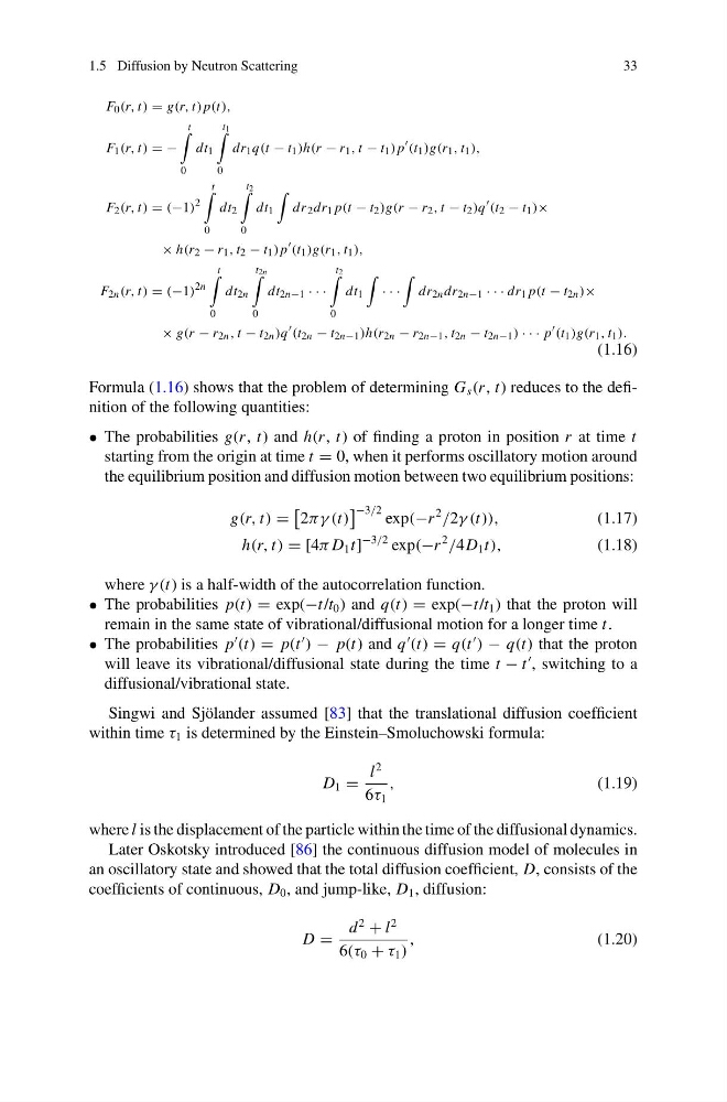
Formula (1.16) shows that the problem of determining G s (r , t) reduces to the definition of the following quantities:
• The probabilities g(r , t) and h(r , t) of finding a proton in position r at time t
starting from the origin at time t = 0, when it performs oscillatory motion around
the equilibrium position and diffusion motion between two equilibrium positions:
g(r, t) =
2πγ (t)
−3/2 exp(−r
2
/2γ (t)),
(1.17)
h(r, t) = [4π D 1 t]
−3/2 exp(−r
2
/4D 1 t),
(1.18)
where γ (t) is a half-width of the autocorrelation function.
• The probabilities p(t) = exp(−t/t 0 ) and q(t) = exp(−t/t 1 ) that the proton will
remain in the same state of vibrational/diffusional motion for a longer time t.
• The probabilities p
(t) = p(t
) − p(t) and q
(t) = q(t
) − q(t) that the proton
will leave its vibrational/diffusional state during the time t − t
, switching to a
diffusional/vibrational state.
Singwi and Sjölander assumed [83] that the translational diffusion coefficient
within time τ 1 is determined by the Einstein–Smoluchowski formula:
D 1 =
l
2
6τ 1
,
(1.19)
where l is the displacement of the particle within the time of the diffusional dynamics.
Later Oskotsky introduced [86] the continuous diffusion model of molecules in
an oscillatory state and showed that the total diffusion coefficient, D, consists of the
coefficients of continuous, D 0 , and jump-like, D 1 , diffusion:
D =
d
2
+ l
2
6(τ 0 + τ 1 )
,
(1.20)
33
F 0 (r, t) = g(r, t) p(t),
F 1 (r, t) = −
t
0
dt 1
t1
0
dr 1 q(t − t 1 )h(r − r 1 , t − t 1 ) p
(t 1 )g(r 1 , t 1 ),
F 2 (r, t) = (−1)
2
t
0
dt 2
t2
0
dt 1
dr 2 dr 1 p(t − t 2 )g(r − r 2 , t − t 2 )q
(t 2 − t 1 )×
× h(r 2 − r 1 , t 2 − t 1 ) p
(t 1 )g(r 1 , t 1 ),
F 2n (r, t) = (−1)
2n
t
0
dt 2n
t2n
0
dt 2n−1 · · ·
t2
0
dt 1
· · ·
dr 2n dr 2n−1 · · · dr 1 p(t − t 2n )×
× g(r − r 2n , t − t 2n )q
(t 2n − t 2n−1 )h(r 2n − r 2n−1 , t 2n − t 2n−1 ) · · · p
(t 1 )g(r 1 , t 1 ).
(1.16)
Formula (1.16) shows that the problem of determining G s (r , t) reduces to the definition of the following quantities:
• The probabilities g(r , t) and h(r , t) of finding a proton in position r at time t
starting from the origin at time t = 0, when it performs oscillatory motion around
the equilibrium position and diffusion motion between two equilibrium positions:
g(r, t) =
2πγ (t)
−3/2 exp(−r
2
/2γ (t)),
(1.17)
h(r, t) = [4π D 1 t]
−3/2 exp(−r
2
/4D 1 t),
(1.18)
where γ (t) is a half-width of the autocorrelation function.
• The probabilities p(t) = exp(−t/t 0 ) and q(t) = exp(−t/t 1 ) that the proton will
remain in the same state of vibrational/diffusional motion for a longer time t.
• The probabilities p
(t) = p(t
) − p(t) and q
(t) = q(t
) − q(t) that the proton
will leave its vibrational/diffusional state during the time t − t
, switching to a
diffusional/vibrational state.
Singwi and Sjölander assumed [83] that the translational diffusion coefficient
within time τ 1 is determined by the Einstein–Smoluchowski formula:
D 1 =
l
2
6τ 1
,
(1.19)
where l is the displacement of the particle within the time of the diffusional dynamics.
Later Oskotsky introduced [86] the continuous diffusion model of molecules in
an oscillatory state and showed that the total diffusion coefficient, D, consists of the
coefficients of continuous, D 0 , and jump-like, D 1 , diffusion:
D =
d
2
+ l
2
6(τ 0 + τ 1 )
,
(1.20)