

5.1 The Dielectric Response of Electrolyte Solutions
187
+
*
(H)Cl
H 3 O
+ → H 2 O
H 2 O → H 3 O
*
j
+
+
(H)Cl
H 3 O
+
H 3 O
+
Proton
exchange
Catalist
=
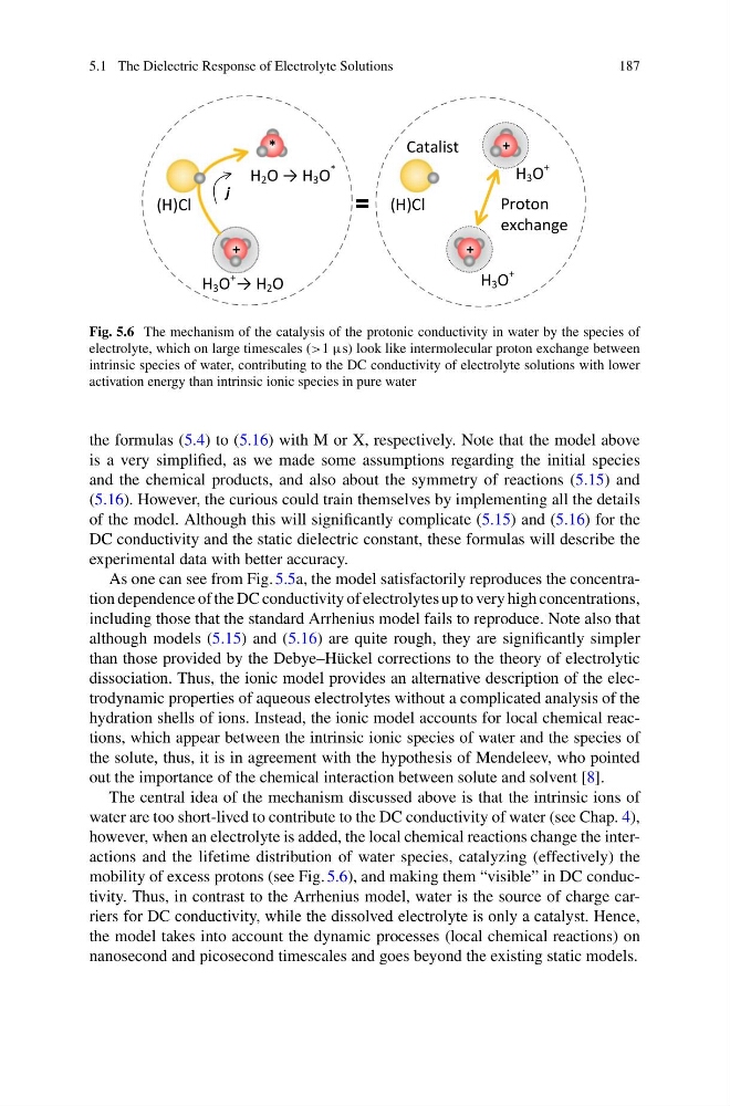
Fig. 5.6 The mechanism of the catalysis of the protonic conductivity in water by the species of
electrolyte, which on large timescales (>1 µs) look like intermolecular proton exchange between
intrinsic species of water, contributing to the DC conductivity of electrolyte solutions with lower
activation energy than intrinsic ionic species in pure water
the formulas (5.4) to (5.16) with M or X, respectively. Note that the model above
is a very simplified, as we made some assumptions regarding the initial species
and the chemical products, and also about the symmetry of reactions (5.15) and
(5.16). However, the curious could train themselves by implementing all the details
of the model. Although this will significantly complicate (5.15) and (5.16) for the
DC conductivity and the static dielectric constant, these formulas will describe the
experimental data with better accuracy.
As one can see from Fig. 5.5a, the model satisfactorily reproduces the concentration dependence of the DC conductivity of electrolytes up to very high concentrations,
including those that the standard Arrhenius model fails to reproduce. Note also that
although models (5.15) and (5.16) are quite rough, they are significantly simpler
than those provided by the Debye–Hückel corrections to the theory of electrolytic
dissociation. Thus, the ionic model provides an alternative description of the electrodynamic properties of aqueous electrolytes without a complicated analysis of the
hydration shells of ions. Instead, the ionic model accounts for local chemical reactions, which appear between the intrinsic ionic species of water and the species of
the solute, thus, it is in agreement with the hypothesis of Mendeleev, who pointed
out the importance of the chemical interaction between solute and solvent [8].
The central idea of the mechanism discussed above is that the intrinsic ions of
water are too short-lived to contribute to the DC conductivity of water (see Chap. 4),
however, when an electrolyte is added, the local chemical reactions change the interactions and the lifetime distribution of water species, catalyzing (effectively) the
mobility of excess protons (see Fig. 5.6), and making them “visible” in DC conductivity. Thus, in contrast to the Arrhenius model, water is the source of charge carriers for DC conductivity, while the dissolved electrolyte is only a catalyst. Hence,
the model takes into account the dynamic processes (local chemical reactions) on
nanosecond and picosecond timescales and goes beyond the existing static models.
187
+
*
(H)Cl
H 3 O
+ → H 2 O
H 2 O → H 3 O
*
j
+
+
(H)Cl
H 3 O
+
H 3 O
+
Proton
exchange
Catalist
=
Fig. 5.6 The mechanism of the catalysis of the protonic conductivity in water by the species of
electrolyte, which on large timescales (>1 µs) look like intermolecular proton exchange between
intrinsic species of water, contributing to the DC conductivity of electrolyte solutions with lower
activation energy than intrinsic ionic species in pure water
the formulas (5.4) to (5.16) with M or X, respectively. Note that the model above
is a very simplified, as we made some assumptions regarding the initial species
and the chemical products, and also about the symmetry of reactions (5.15) and
(5.16). However, the curious could train themselves by implementing all the details
of the model. Although this will significantly complicate (5.15) and (5.16) for the
DC conductivity and the static dielectric constant, these formulas will describe the
experimental data with better accuracy.
As one can see from Fig. 5.5a, the model satisfactorily reproduces the concentration dependence of the DC conductivity of electrolytes up to very high concentrations,
including those that the standard Arrhenius model fails to reproduce. Note also that
although models (5.15) and (5.16) are quite rough, they are significantly simpler
than those provided by the Debye–Hückel corrections to the theory of electrolytic
dissociation. Thus, the ionic model provides an alternative description of the electrodynamic properties of aqueous electrolytes without a complicated analysis of the
hydration shells of ions. Instead, the ionic model accounts for local chemical reactions, which appear between the intrinsic ionic species of water and the species of
the solute, thus, it is in agreement with the hypothesis of Mendeleev, who pointed
out the importance of the chemical interaction between solute and solvent [8].
The central idea of the mechanism discussed above is that the intrinsic ions of
water are too short-lived to contribute to the DC conductivity of water (see Chap. 4),
however, when an electrolyte is added, the local chemical reactions change the interactions and the lifetime distribution of water species, catalyzing (effectively) the
mobility of excess protons (see Fig. 5.6), and making them “visible” in DC conductivity. Thus, in contrast to the Arrhenius model, water is the source of charge carriers for DC conductivity, while the dissolved electrolyte is only a catalyst. Hence,
the model takes into account the dynamic processes (local chemical reactions) on
nanosecond and picosecond timescales and goes beyond the existing static models.