

126
3 The Interaction of Electromagnetic Waves with Ice
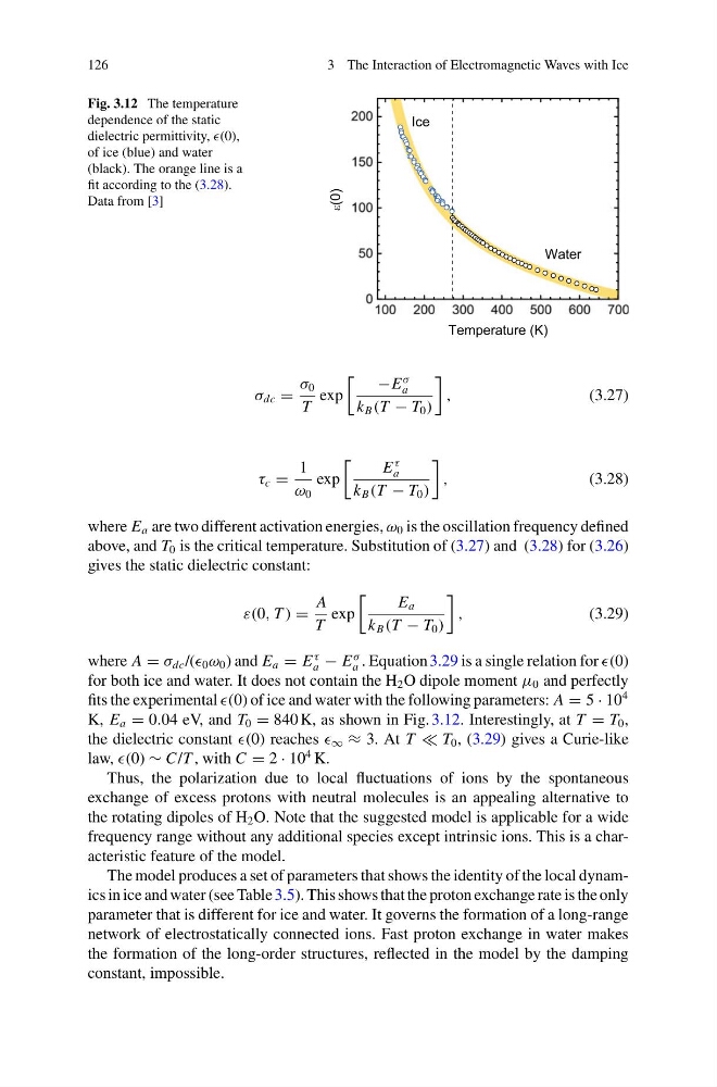
Fig. 3.12 The temperature
dependence of the static
dielectric permittivity, (0),
of ice (blue) and water
(black). The orange line is a
fit according to the (3.28).
Data from [3]
σ dc =
σ 0
T
exp
−E
σ
a
k B (T − T 0 )
,
(3.27)
τ c =
1
ω 0
exp
E
τ
a
k B (T − T 0 )
,
(3.28)
where E a are two different activation energies, ω 0 is the oscillation frequency defined
above, and T 0 is the critical temperature. Substitution of (3.27) and (3.28) for (3.26)
gives the static dielectric constant:
ε(0, T ) =
A
T
exp
E a
k B (T − T 0 )
,
(3.29)
where A = σ dc /( 0 ω 0 ) and E a = E
τ
a − E
σ
a . Equation 3.29 is a single relation for (0)
for both ice and water. It does not contain the H 2 O dipole moment μ 0 and perfectly
fits the experimental (0) of ice and water with the following parameters: A = 5 · 10
4
K, E a = 0.04 eV, and T 0 = 840 K, as shown in Fig. 3.12. Interestingly, at T = T 0 ,
the dielectric constant (0) reaches ∞ ≈ 3. At T T 0 , (3.29) gives a Curie-like
law, (0) ∼ C/T , with C = 2 · 10
4 K.
Thus, the polarization due to local fluctuations of ions by the spontaneous
exchange of excess protons with neutral molecules is an appealing alternative to
the rotating dipoles of H 2 O. Note that the suggested model is applicable for a wide
frequency range without any additional species except intrinsic ions. This is a characteristic feature of the model.
The model produces a set of parameters that shows the identity of the local dynamics in ice and water (see Table 3.5). This shows that the proton exchange rate is the only
parameter that is different for ice and water. It governs the formation of a long-range
network of electrostatically connected ions. Fast proton exchange in water makes
the formation of the long-order structures, reflected in the model by the damping
constant, impossible.
3 The Interaction of Electromagnetic Waves with Ice
Fig. 3.12 The temperature
dependence of the static
dielectric permittivity, (0),
of ice (blue) and water
(black). The orange line is a
fit according to the (3.28).
Data from [3]
σ dc =
σ 0
T
exp
−E
σ
a
k B (T − T 0 )
,
(3.27)
τ c =
1
ω 0
exp
E
τ
a
k B (T − T 0 )
,
(3.28)
where E a are two different activation energies, ω 0 is the oscillation frequency defined
above, and T 0 is the critical temperature. Substitution of (3.27) and (3.28) for (3.26)
gives the static dielectric constant:
ε(0, T ) =
A
T
exp
E a
k B (T − T 0 )
,
(3.29)
where A = σ dc /( 0 ω 0 ) and E a = E
τ
a − E
σ
a . Equation 3.29 is a single relation for (0)
for both ice and water. It does not contain the H 2 O dipole moment μ 0 and perfectly
fits the experimental (0) of ice and water with the following parameters: A = 5 · 10
4
K, E a = 0.04 eV, and T 0 = 840 K, as shown in Fig. 3.12. Interestingly, at T = T 0 ,
the dielectric constant (0) reaches ∞ ≈ 3. At T T 0 , (3.29) gives a Curie-like
law, (0) ∼ C/T , with C = 2 · 10
4 K.
Thus, the polarization due to local fluctuations of ions by the spontaneous
exchange of excess protons with neutral molecules is an appealing alternative to
the rotating dipoles of H 2 O. Note that the suggested model is applicable for a wide
frequency range without any additional species except intrinsic ions. This is a characteristic feature of the model.
The model produces a set of parameters that shows the identity of the local dynamics in ice and water (see Table 3.5). This shows that the proton exchange rate is the only
parameter that is different for ice and water. It governs the formation of a long-range
network of electrostatically connected ions. Fast proton exchange in water makes
the formation of the long-order structures, reflected in the model by the damping
constant, impossible.