

112
3 The Interaction of Electromagnetic Waves with Ice
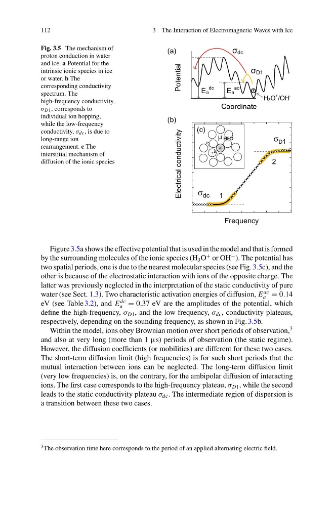
Fig. 3.5 The mechanism of
proton conduction in water
and ice. a Potential for the
intrinsic ionic species in ice
or water. b The
corresponding conductivity
spectrum. The
high-frequency conductivity,
σ D1 , corresponds to
individual ion hopping,
while the low-frequency
conductivity, σ dc , is due to
long-range ion
rearrangement. c The
interstitial mechanism of
diffusion of the ionic species
Potential
(a)
(b)
Coordinate
H 3 O
+ /OH
-
σ D1
σ dc
E a
ac
E a
dc
+
+
dc
Electrical conductivity
Frequency
D1
1
2
(c)
μ H2O
Figure 3.5a shows the effective potential that is used in the model and that is formed
by the surrounding molecules of the ionic species (H 3 O
+ or OH
− ). The potential has
two spatial periods, one is due to the nearest molecular species (see Fig. 3.5c), and the
other is because of the electrostatic interaction with ions of the opposite charge. The
latter was previously neglected in the interpretation of the static conductivity of pure
water (see Sect. 1.3). Two characteristic activation energies of diffusion, E
ac
a = 0.14
eV (see Table 3.2), and E
dc
a = 0.37 eV are the amplitudes of the potential, which
define the high-frequency, σ D1 , and the low frequency, σ dc , conductivity plateaus,
respectively, depending on the sounding frequency, as shown in Fig. 3.5b.
Within the model, ions obey Brownian motion over short periods of observation,
3
and also at very long (more than 1 µs) periods of observation (the static regime).
However, the diffusion coefficients (or mobilities) are different for these two cases.
The short-term diffusion limit (high frequencies) is for such short periods that the
mutual interaction between ions can be neglected. The long-term diffusion limit
(very low frequencies) is, on the contrary, for the ambipolar diffusion of interacting
ions. The first case corresponds to the high-frequency plateau, σ D1 , while the second
leads to the static conductivity plateau σ dc . The intermediate region of dispersion is
a transition between these two cases.
3 The observation time here corresponds to the period of an applied alternating electric field.
3 The Interaction of Electromagnetic Waves with Ice
Fig. 3.5 The mechanism of
proton conduction in water
and ice. a Potential for the
intrinsic ionic species in ice
or water. b The
corresponding conductivity
spectrum. The
high-frequency conductivity,
σ D1 , corresponds to
individual ion hopping,
while the low-frequency
conductivity, σ dc , is due to
long-range ion
rearrangement. c The
interstitial mechanism of
diffusion of the ionic species
Potential
(a)
(b)
Coordinate
H 3 O
+ /OH
-
σ D1
σ dc
E a
ac
E a
dc
+
+
dc
Electrical conductivity
Frequency
D1
1
2
(c)
μ H2O
Figure 3.5a shows the effective potential that is used in the model and that is formed
by the surrounding molecules of the ionic species (H 3 O
+ or OH
− ). The potential has
two spatial periods, one is due to the nearest molecular species (see Fig. 3.5c), and the
other is because of the electrostatic interaction with ions of the opposite charge. The
latter was previously neglected in the interpretation of the static conductivity of pure
water (see Sect. 1.3). Two characteristic activation energies of diffusion, E
ac
a = 0.14
eV (see Table 3.2), and E
dc
a = 0.37 eV are the amplitudes of the potential, which
define the high-frequency, σ D1 , and the low frequency, σ dc , conductivity plateaus,
respectively, depending on the sounding frequency, as shown in Fig. 3.5b.
Within the model, ions obey Brownian motion over short periods of observation,
3
and also at very long (more than 1 µs) periods of observation (the static regime).
However, the diffusion coefficients (or mobilities) are different for these two cases.
The short-term diffusion limit (high frequencies) is for such short periods that the
mutual interaction between ions can be neglected. The long-term diffusion limit
(very low frequencies) is, on the contrary, for the ambipolar diffusion of interacting
ions. The first case corresponds to the high-frequency plateau, σ D1 , while the second
leads to the static conductivity plateau σ dc . The intermediate region of dispersion is
a transition between these two cases.
3 The observation time here corresponds to the period of an applied alternating electric field.