

32
Biomedical Signal and Image Processing
50
100
150
200
250
300
y
50
100
150
200
250
300
350
x
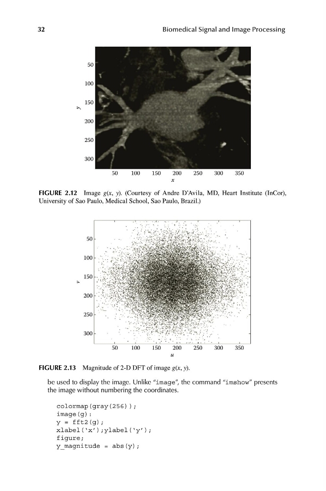
FIGURE 2.12 Image g(x, y). (Courtesy of Andre D’Avila, MD, Heart Institute (InCor),
University of Sao Paulo, Medical School, Sao Paulo, Brazil.)
50
100
150
200
250
300
v
50
100
150
200
250
300
350
u
FIGURE 2.13 Magnitude of 2-D DFT of image g(x, y).
be used to display the image. Unlike “image”, the command “imshow” presents
the image without numbering the coordinates.
colormap(gray(256) );
image(g):
y = fft2(g);
xlabel(‘x’);ylabel(‘y’);
figure;
y_magnitude = abs(y);
Biomedical Signal and Image Processing
50
100
150
200
250
300
y
50
100
150
200
250
300
350
x
FIGURE 2.12 Image g(x, y). (Courtesy of Andre D’Avila, MD, Heart Institute (InCor),
University of Sao Paulo, Medical School, Sao Paulo, Brazil.)
50
100
150
200
250
300
v
50
100
150
200
250
300
350
u
FIGURE 2.13 Magnitude of 2-D DFT of image g(x, y).
be used to display the image. Unlike “image”, the command “imshow” presents
the image without numbering the coordinates.
colormap(gray(256) );
image(g):
y = fft2(g);
xlabel(‘x’);ylabel(‘y’);
figure;
y_magnitude = abs(y);