

16
Biomedical Signal and Image Processing
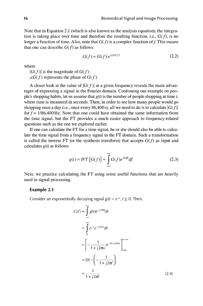
Note that in Equation 2.1 (which is also known as the analysis equation), the integration is taking place over time and therefore the resulting function, i.e., G( f), is no
longer a function of time. Also, note that G( f) is a complex function of f. This means
that one can describe G( f) as follows:
∠ ( )
e
j G f
(2.2)
G f =
( ) G f
( )
where
�G( f )� is the magnitude of G( f )
∠G( f ) represents the phase of G( f )
A closer look at the value of �G( f )� at a given frequency reveals the main advantages of expressing a signal in the Fourier domain. Continuing our example on people’s shopping habits, let us assume that g(t) is the number of people shopping at time t,
where time is measured in seconds. Then, in order to see how many people would go
shopping once a day (i.e., once every 86,400 s), all we need to do is to calculate �G( f)�
for f = 1/86,400 Hz. Note that one could have obtained the same information from
the time signal, but the FT provides a much easier approach to frequency-related
questions such as the one we explored earlier.
If one can calculate the FT for a time signal, he or she should also be able to calculate the time signal from a frequency signal in the FT domain. Such a transformation
is called the inverse FT (or the synthesis transform) that accepts G( f) as input and
calculates g(t) as follows:
+∞
g t
( ) = IFT { G( )
f } = ∫
G( )
f e
j f
2p t df
(2.3)
−∞
Next, we practice calculating the FT using some useful functions that are heavily
used in signal processing.
Example 2.1
Consider an exponentially decaying signal g(t) = e −t , t ≥ 0. Then,
+∞
G f
( ) =
∫
g t
( )e
− j 2 pft dt
−∞
+∞
=
∫
e e
−t − j 2p ft dt
0
⎡
t =+∞
1
− +
⎤
= −
⎢
e
( 1 2
j f
p ) )t ⎥
⎣ 1 + j u
2p
⎦ t =0
⎛
1 ⎞
= ( )
0 − −
⎜ ⎝ 1 + j f
2p ⎟ ⎠
1
=
(2.4)
1 + j f
2p
Biomedical Signal and Image Processing
Note that in Equation 2.1 (which is also known as the analysis equation), the integration is taking place over time and therefore the resulting function, i.e., G( f), is no
longer a function of time. Also, note that G( f) is a complex function of f. This means
that one can describe G( f) as follows:
∠ ( )
e
j G f
(2.2)
G f =
( ) G f
( )
where
�G( f )� is the magnitude of G( f )
∠G( f ) represents the phase of G( f )
A closer look at the value of �G( f )� at a given frequency reveals the main advantages of expressing a signal in the Fourier domain. Continuing our example on people’s shopping habits, let us assume that g(t) is the number of people shopping at time t,
where time is measured in seconds. Then, in order to see how many people would go
shopping once a day (i.e., once every 86,400 s), all we need to do is to calculate �G( f)�
for f = 1/86,400 Hz. Note that one could have obtained the same information from
the time signal, but the FT provides a much easier approach to frequency-related
questions such as the one we explored earlier.
If one can calculate the FT for a time signal, he or she should also be able to calculate the time signal from a frequency signal in the FT domain. Such a transformation
is called the inverse FT (or the synthesis transform) that accepts G( f) as input and
calculates g(t) as follows:
+∞
g t
( ) = IFT { G( )
f } = ∫
G( )
f e
j f
2p t df
(2.3)
−∞
Next, we practice calculating the FT using some useful functions that are heavily
used in signal processing.
Example 2.1
Consider an exponentially decaying signal g(t) = e −t , t ≥ 0. Then,
+∞
G f
( ) =
∫
g t
( )e
− j 2 pft dt
−∞
+∞
=
∫
e e
−t − j 2p ft dt
0
⎡
t =+∞
1
− +
⎤
= −
⎢
e
( 1 2
j f
p ) )t ⎥
⎣ 1 + j u
2p
⎦ t =0
⎛
1 ⎞
= ( )
0 − −
⎜ ⎝ 1 + j f
2p ⎟ ⎠
1
=
(2.4)
1 + j f
2p