

147
Clustering and Classification
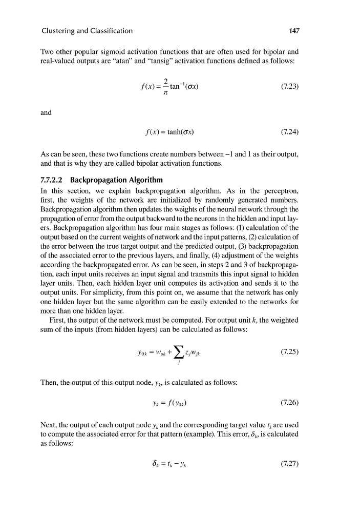
Two other popular sigmoid activation functions that are often used for bipolar and
real-valued outputs are “atan” and “tansig” activation functions defined as follows:
2
−1
f x = tan ( x
( )
s )
(7.23)
p
and
f x
( ) = tanh(sx)
(7.24)
As can be seen, these two functions create numbers between −1 and 1 as their output,
and that is why they are called bipolar activation functions.
7.7.2.2 Backpropagation Algorithm
In this section, we explain backpropagation algorithm. As in the perceptron,
first, the weights of the network are initialized by randomly generated numbers.
Backpropagation algorithm then updates the weights of the neural network through the
propagation of error from the output backward to the neurons in the hidden and input layers. Backpropagation algorithm has four main stages as follows: (1) calculation of the
output based on the current weights of network and the input patterns, (2) calculation of
the error between the true target output and the predicted output, (3) backpropagation
of the associated error to the previous layers, and finally, (4) adjustment of the weights
according the backpropagated error. As can be seen, in steps 2 and 3 of backpropagation, each input units receives an input signal and transmits this input signal to hidden
layer units. Then, each hidden layer unit computes its activation and sends it to the
output units. For simplicity, from this point on, we assume that the network has only
one hidden layer but the same algorithm can be easily extended to the networks for
more than one hidden layer.
First, the output of the network must be computed. For output unit k, the weighted
sum of the inputs (from hidden layers) can be calculated as follows:
y = w + ∑ z w
(7.25)
0 k
o k
j j k
j
Then, the output of this output node, y k , is calculated as follows:
y k = f y 0k
( )
(7.26)
Next, the output of each output node y k and the corresponding target value t k are used
to compute the associated error for that pattern (example). This error, δ k , is calculated
as follows:
d k = −
t k y k
(7.27)
Clustering and Classification
Two other popular sigmoid activation functions that are often used for bipolar and
real-valued outputs are “atan” and “tansig” activation functions defined as follows:
2
−1
f x = tan ( x
( )
s )
(7.23)
p
and
f x
( ) = tanh(sx)
(7.24)
As can be seen, these two functions create numbers between −1 and 1 as their output,
and that is why they are called bipolar activation functions.
7.7.2.2 Backpropagation Algorithm
In this section, we explain backpropagation algorithm. As in the perceptron,
first, the weights of the network are initialized by randomly generated numbers.
Backpropagation algorithm then updates the weights of the neural network through the
propagation of error from the output backward to the neurons in the hidden and input layers. Backpropagation algorithm has four main stages as follows: (1) calculation of the
output based on the current weights of network and the input patterns, (2) calculation of
the error between the true target output and the predicted output, (3) backpropagation
of the associated error to the previous layers, and finally, (4) adjustment of the weights
according the backpropagated error. As can be seen, in steps 2 and 3 of backpropagation, each input units receives an input signal and transmits this input signal to hidden
layer units. Then, each hidden layer unit computes its activation and sends it to the
output units. For simplicity, from this point on, we assume that the network has only
one hidden layer but the same algorithm can be easily extended to the networks for
more than one hidden layer.
First, the output of the network must be computed. For output unit k, the weighted
sum of the inputs (from hidden layers) can be calculated as follows:
y = w + ∑ z w
(7.25)
0 k
o k
j j k
j
Then, the output of this output node, y k , is calculated as follows:
y k = f y 0k
( )
(7.26)
Next, the output of each output node y k and the corresponding target value t k are used
to compute the associated error for that pattern (example). This error, δ k , is calculated
as follows:
d k = −
t k y k
(7.27)