144
Biomedical Signal and Image Processing
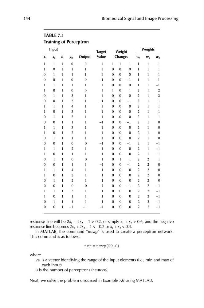
TABLE 7.1
Training of Perceptron
Input
Target
Weight
Weights
x 1
x 2
b
y 0
Output
Value
Changes
w 1
w 2
w 3
1
1
1
0
0
1
1 1
1
1
1
1
1
0
1
1
1
1
0 0
0
1
1
1
0
1
1
1
1
1
0 0
0
1
1
1
0
0
1
0
0
−1
0 0
−1
1
1
−1
1
1
1
1
1
1
0 0
0
1
1
−1
1
0
1
0
0
1
1 0
1
2
1
2
0
1
1
3
1
1
0 0
0
2
1
2
0
0
1
2
1
−1
0 0
−1
2
1
1
1
1
1
4
1
1
0 0
0
2
1
1
1
0
1
3
1
1
0 0
0
2
1
1
0
1
1
2
1
1
0 0
0
2
1
1
0
0
1
1
1
−1
0 0
−1
2
1
0
1
1
1
3
1
1
0 0
0
2
1
0
1
0
1
2
1
1
0 0
0
2
1
0
0
1
1
1
1
1
0 0
0
2
1
0
0
0
1
0
0
−1
0 0
−1
2
1
−1
1
1
1
2
1
1
0 0
0
2
1
−1
1
0
1
1
1
1
0 0
0
2
1
−1
0
1
1
0
0
1
0 1
1
2
2
1
0
0
1
1
1
−1
0 0
−1
2
2
0
1
1
1
4
1
1
0 0
0
2
2
0
1
0
1
2
1
1
0 0
0
2
2
0
0
1
1
2
1
1
0 0
0
2
2
0
0
0
1
0
0
−1
0 0
−1
2
2
−1
1
1
1
3
1
1
0 0
0
2
2
−1
1
0
1
1
1
1
0 0
0
2
2
−1
0
1
1
1
1
1
0 0
0
2
2
−1
0
0
1
−1
−1
−1
0 0
0
2
2
−1
response line will be 2x 1 + 2x 2 − 1 > 0.2, or simply x 1 + x 2 > 0.6, and the negative
response line becomes 2x 1 + 2x 2 − 1 < −0.2 or x 1 + x 2 < 0.4.
In MATLAB, the command “newp” is used to create a perceptron network.
This command is as follows:
net = newp(PR,S)
where
PR is a vector identifying the range of the input elements (i.e., min and max of
each input)
S is the number of perceptrons (neurons)
Next, we solve the problem discussed in Example 7.6 using MATLAB.