

137
Clustering and Classification
4
3
2
1
0
–1
–2
–3
–5
–4
–5
–4
– 3
– 2
– 1
0
1
2
3
4
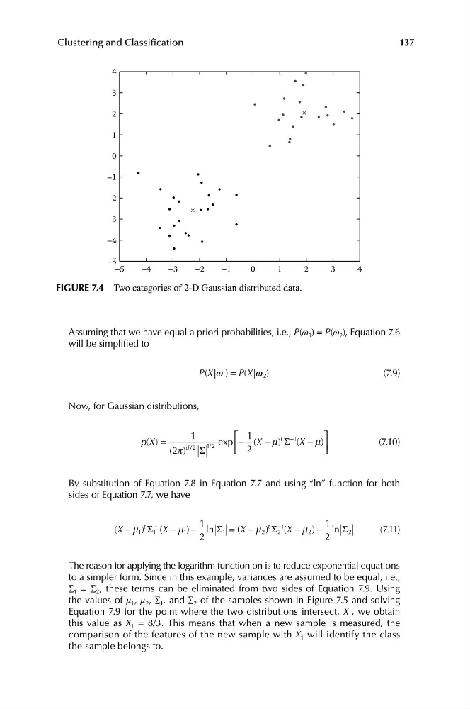
FIGURE 7.4 Two categories of 2-D Gaussian distributed data.
Assuming that we have equal a priori probabilities, i.e., P(ω 1 ) = P(ω 2 ), Equation 7.6
will be simplified to
P X
( |w 1 ) = P X
( |w )
2
(7.9)
Now, for Gaussian distributions,
1
⎡ 1
⎤
p X
( ) =
1 2
/ exp − (X − m )
t Σ
−1
(X − m )
(7.10)
( )
2 p
d / 2
⎢
⎥
Σ
⎣ 2
⎦
By substitution of Equation 7.8 in Equation 7.7 and using “ln” function for both
sides of Equation 7.7, we have
(X − m )
t −1
1
1
1 Σ 1 (X − m
t −1
1 ) − ln Σ 1 = (X − m 2 ) Σ 2 (X − m 2 ) − ln Σ 2
(7.11)
2
2
The reason for applying the logarithm function on is to reduce exponential equations
to a simpler form. Since in this example, variances are assumed to be equal, i.e.,
∑ 1 = ∑ 2 , these terms can be eliminated from two sides of Equation 7.9. Using
the values of μ 1 , μ 2 , ∑ 1 , and ∑ 2 of the samples shown in Figure 7.5 and solving
Equation 7.9 for the point where the two distributions intersect, X 1 , we obtain
this value as X 1 = 8/3. This means that when a new sample is measured, the
comparison of the features of the new sample with X 1 will identify the class
the sample belongs to.
Clustering and Classification
4
3
2
1
0
–1
–2
–3
–5
–4
–5
–4
– 3
– 2
– 1
0
1
2
3
4
FIGURE 7.4 Two categories of 2-D Gaussian distributed data.
Assuming that we have equal a priori probabilities, i.e., P(ω 1 ) = P(ω 2 ), Equation 7.6
will be simplified to
P X
( |w 1 ) = P X
( |w )
2
(7.9)
Now, for Gaussian distributions,
1
⎡ 1
⎤
p X
( ) =
1 2
/ exp − (X − m )
t Σ
−1
(X − m )
(7.10)
( )
2 p
d / 2
⎢
⎥
Σ
⎣ 2
⎦
By substitution of Equation 7.8 in Equation 7.7 and using “ln” function for both
sides of Equation 7.7, we have
(X − m )
t −1
1
1
1 Σ 1 (X − m
t −1
1 ) − ln Σ 1 = (X − m 2 ) Σ 2 (X − m 2 ) − ln Σ 2
(7.11)
2
2
The reason for applying the logarithm function on is to reduce exponential equations
to a simpler form. Since in this example, variances are assumed to be equal, i.e.,
∑ 1 = ∑ 2 , these terms can be eliminated from two sides of Equation 7.9. Using
the values of μ 1 , μ 2 , ∑ 1 , and ∑ 2 of the samples shown in Figure 7.5 and solving
Equation 7.9 for the point where the two distributions intersect, X 1 , we obtain
this value as X 1 = 8/3. This means that when a new sample is measured, the
comparison of the features of the new sample with X 1 will identify the class
the sample belongs to.