

sensors and the logger for roughly 3 month together with an autonomous underwater tide and wave recorder (RBR TWR-2050). The tide and wave recorder was
used, to meet exact statements about the arising wave spectra during the test period.
Data noted during the trial period were acquired all 30 min in one burst with a 512
sample measurement length and were averaged afterwards. This power saving
strategy allowed for a time span of approx. 3 months before the inbuilt batteries
were exhausted.
Measurements of currents in the plane of the collectors, approx. 7 m below
water surface was achieved by applying a current meter (AADI RCM-9LW) at a
mooring site in approximately 30 m distance from the longline demonstrator. The
current meter was additionally equipped with pressure, temperature and conductivity sensors to address the oceanographic conditions as well as a turbidity probe
and a shallow water oxygen sensor, both to account for growth parameters of the
biological setup. Due to the high capacity of the RCM-9LW batteries no power
saving precautions had to been taken and a sample interval of 10 min was realized.
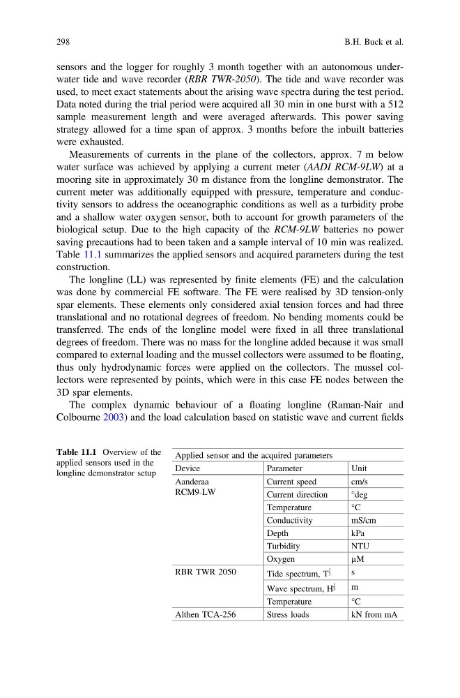
Table 11.1 summarizes the applied sensors and acquired parameters during the test
construction.
The longline (LL) was represented by finite elements (FE) and the calculation
was done by commercial FE software. The FE were realised by 3D tension-only
spar elements. These elements only considered axial tension forces and had three
translational and no rotational degrees of freedom. No bending moments could be
transferred. The ends of the longline model were fixed in all three translational
degrees of freedom. There was no mass for the longline added because it was small
compared to external loading and the mussel collectors were assumed to be floating,
thus only hydrodynamic forces were applied on the collectors. The mussel collectors were represented by points, which were in this case FE nodes between the
3D spar elements.
The complex dynamic behaviour of a floating longline (Raman-Nair and
Colbourne 2003) and the load calculation based on statistic wave and current fields
Table 11.1 Overview of the
applied sensors used in the
longline demonstrator setup
Applied sensor and the acquired parameters
Device
Parameter
Unit
Aanderaa
RCM9-LW
Current speed
cm/s
Current direction
°deg
Temperature
°C
Conductivity
mS/cm
Depth
kPa
Turbidity
NTU
Oxygen
µM
RBR TWR 2050
Tide spectrum, T
1
3
s
Wave spectrum, H
1
3
m
Temperature
°C
Althen TCA-256
Stress loads
kN from mA
298
B.H. Buck et al.
used, to meet exact statements about the arising wave spectra during the test period.
Data noted during the trial period were acquired all 30 min in one burst with a 512
sample measurement length and were averaged afterwards. This power saving
strategy allowed for a time span of approx. 3 months before the inbuilt batteries
were exhausted.
Measurements of currents in the plane of the collectors, approx. 7 m below
water surface was achieved by applying a current meter (AADI RCM-9LW) at a
mooring site in approximately 30 m distance from the longline demonstrator. The
current meter was additionally equipped with pressure, temperature and conductivity sensors to address the oceanographic conditions as well as a turbidity probe
and a shallow water oxygen sensor, both to account for growth parameters of the
biological setup. Due to the high capacity of the RCM-9LW batteries no power
saving precautions had to been taken and a sample interval of 10 min was realized.
Table 11.1 summarizes the applied sensors and acquired parameters during the test
construction.
The longline (LL) was represented by finite elements (FE) and the calculation
was done by commercial FE software. The FE were realised by 3D tension-only
spar elements. These elements only considered axial tension forces and had three
translational and no rotational degrees of freedom. No bending moments could be
transferred. The ends of the longline model were fixed in all three translational
degrees of freedom. There was no mass for the longline added because it was small
compared to external loading and the mussel collectors were assumed to be floating,
thus only hydrodynamic forces were applied on the collectors. The mussel collectors were represented by points, which were in this case FE nodes between the
3D spar elements.
The complex dynamic behaviour of a floating longline (Raman-Nair and
Colbourne 2003) and the load calculation based on statistic wave and current fields
Table 11.1 Overview of the
applied sensors used in the
longline demonstrator setup
Applied sensor and the acquired parameters
Device
Parameter
Unit
Aanderaa
RCM9-LW
Current speed
cm/s
Current direction
°deg
Temperature
°C
Conductivity
mS/cm
Depth
kPa
Turbidity
NTU
Oxygen
µM
RBR TWR 2050
Tide spectrum, T
1
3
s
Wave spectrum, H
1
3
m
Temperature
°C
Althen TCA-256
Stress loads
kN from mA
298
B.H. Buck et al.