

4.1 What Is Nonlinear Optics?
85
∇
2 ˜
E −
0 c 2
∂
2 ˜
E
∂t 2 = 0
(4.12)
Absorbing the into the differential, we get
∇
2 ˜
E −
1
0 c 2
∂
2 ˜
D
∂t 2 = 0
(4.13)
Now, since ˜
D = 0 ˜
E + ˜
P
(1) + ˜
P
N L (from Eqs. 1.2, 1.3, 1.4, and 1.8), wave equation
becomes
∇
2 ˜
E −
1
0 c 2
∂
2 ˜
D
(1)
∂t 2 =
1
0 c 2
∂
2 ˜
P
N L
∂t 2
(4.14)
or
∇
2 ˜
E −
(1)
c 2
∂
2 ˜
E
∂t 2 =
1
0 c 2
∂
2 ˜
P
N L
∂t 2
(4.15)
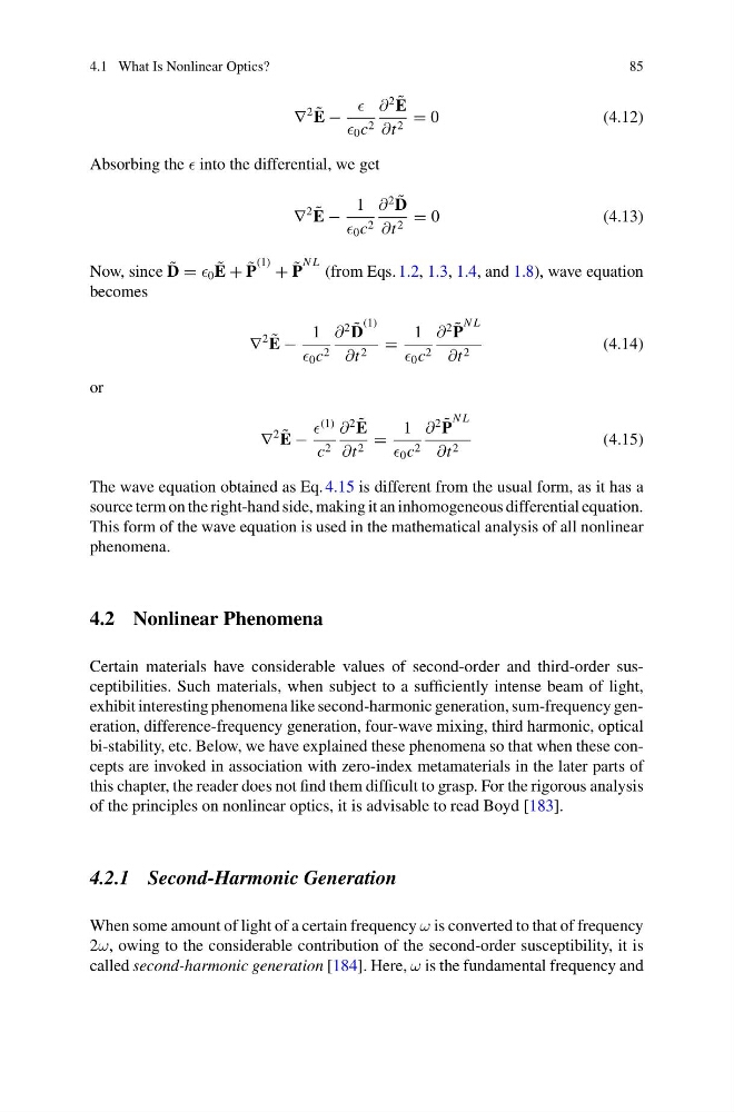
The wave equation obtained as Eq. 4.15 is different from the usual form, as it has a
source term on the right-hand side, making it an inhomogeneous differential equation.
This form of the wave equation is used in the mathematical analysis of all nonlinear
phenomena.
4.2 Nonlinear Phenomena
Certain materials have considerable values of second-order and third-order susceptibilities. Such materials, when subject to a sufficiently intense beam of light,
exhibit interesting phenomena like second-harmonic generation, sum-frequency generation, difference-frequency generation, four-wave mixing, third harmonic, optical
bi-stability, etc. Below, we have explained these phenomena so that when these concepts are invoked in association with zero-index metamaterials in the later parts of
this chapter, the reader does not find them difficult to grasp. For the rigorous analysis
of the principles on nonlinear optics, it is advisable to read Boyd [183].
4.2.1 Second-Harmonic Generation
When some amount of light of a certain frequency ω is converted to that of frequency
2ω, owing to the considerable contribution of the second-order susceptibility, it is
called second-harmonic generation [184]. Here, ω is the fundamental frequency and
85
∇
2 ˜
E −
0 c 2
∂
2 ˜
E
∂t 2 = 0
(4.12)
Absorbing the into the differential, we get
∇
2 ˜
E −
1
0 c 2
∂
2 ˜
D
∂t 2 = 0
(4.13)
Now, since ˜
D = 0 ˜
E + ˜
P
(1) + ˜
P
N L (from Eqs. 1.2, 1.3, 1.4, and 1.8), wave equation
becomes
∇
2 ˜
E −
1
0 c 2
∂
2 ˜
D
(1)
∂t 2 =
1
0 c 2
∂
2 ˜
P
N L
∂t 2
(4.14)
or
∇
2 ˜
E −
(1)
c 2
∂
2 ˜
E
∂t 2 =
1
0 c 2
∂
2 ˜
P
N L
∂t 2
(4.15)
The wave equation obtained as Eq. 4.15 is different from the usual form, as it has a
source term on the right-hand side, making it an inhomogeneous differential equation.
This form of the wave equation is used in the mathematical analysis of all nonlinear
phenomena.
4.2 Nonlinear Phenomena
Certain materials have considerable values of second-order and third-order susceptibilities. Such materials, when subject to a sufficiently intense beam of light,
exhibit interesting phenomena like second-harmonic generation, sum-frequency generation, difference-frequency generation, four-wave mixing, third harmonic, optical
bi-stability, etc. Below, we have explained these phenomena so that when these concepts are invoked in association with zero-index metamaterials in the later parts of
this chapter, the reader does not find them difficult to grasp. For the rigorous analysis
of the principles on nonlinear optics, it is advisable to read Boyd [183].
4.2.1 Second-Harmonic Generation
When some amount of light of a certain frequency ω is converted to that of frequency
2ω, owing to the considerable contribution of the second-order susceptibility, it is
called second-harmonic generation [184]. Here, ω is the fundamental frequency and