

6.4 Exposure Assessment (Step 2)
127
environmental concentrations in the various compartments. They have the ability
to describe the processes of:
• Mass transport within an environmental compartment: Through convective
mixing, a substance can move according to the flow of the corresponding
environmental medium (air, water) within a compartment.
• Mass transport between environmental compartments: Through mass flow across
media boundaries, the substance passes into other environmental compartments,
e.g., by diffusion (evaporation), advective outflow, etc.
• Substance transformation through biotic degradation: Substances can be biologically converted, for example, by microorganisms in the soil or water.
• Substance transformation by abiotic degradation: Hydrolysis, photolysis, oxidation, etc. can cause chemical transformation.
• Sorption: Substances can be sorbed onto particles in soils, waters, and sediments.
This leads to them becoming enriched and retained in that compartment.
• Bioaccumulation: Substances can accumulate in organisms along the food chain
(particularly hydrophobic substances).
As outlined in Fig. 6.12, the modeling of these processes requires three types
of data for input into a mass-balance model: emission data, substance data, and
environmental data.
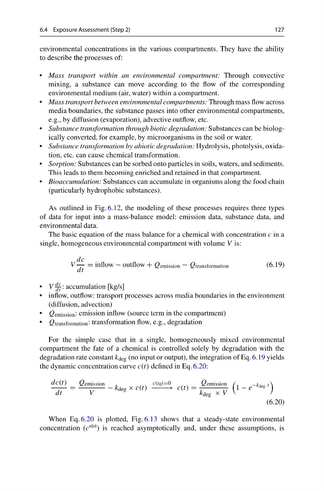
The basic equation of the mass balance for a chemical with concentration c in a
single, homogeneous environmental compartment with volume V is:
V
dc
dt
= inflow − outflow + Q emission − Q transformation
(6.19)
• V
dc
dt : accumulation [kg/s]
• inflow, outflow: transport processes across media boundaries in the environment
(diffusion, advection)
• Q emission : emission inflow (source term in the compartment)
• Q transformation : transformation flow, e.g., degradation
For the simple case that in a single, homogeneously mixed environmental
compartment the fate of a chemical is controlled solely by degradation with the
degradation rate constant k deg (no input or output), the integration of Eq. 6.19 yields
the dynamic concentration curve c(t) defined in Eq. 6.20:
dc(t)
dt
=
Q emission
V
− k deg × c(t)
c(t 0 )=0
− −−− → c(t) =
Q emission
k deg × V
1 − e
−k deg t
(6.20)
When Eq. 6.20 is plotted, Fig. 6.13 shows that a steady-state environmental
concentration (c stst ) is reached asymptotically and, under these assumptions, is
127
environmental concentrations in the various compartments. They have the ability
to describe the processes of:
• Mass transport within an environmental compartment: Through convective
mixing, a substance can move according to the flow of the corresponding
environmental medium (air, water) within a compartment.
• Mass transport between environmental compartments: Through mass flow across
media boundaries, the substance passes into other environmental compartments,
e.g., by diffusion (evaporation), advective outflow, etc.
• Substance transformation through biotic degradation: Substances can be biologically converted, for example, by microorganisms in the soil or water.
• Substance transformation by abiotic degradation: Hydrolysis, photolysis, oxidation, etc. can cause chemical transformation.
• Sorption: Substances can be sorbed onto particles in soils, waters, and sediments.
This leads to them becoming enriched and retained in that compartment.
• Bioaccumulation: Substances can accumulate in organisms along the food chain
(particularly hydrophobic substances).
As outlined in Fig. 6.12, the modeling of these processes requires three types
of data for input into a mass-balance model: emission data, substance data, and
environmental data.
The basic equation of the mass balance for a chemical with concentration c in a
single, homogeneous environmental compartment with volume V is:
V
dc
dt
= inflow − outflow + Q emission − Q transformation
(6.19)
• V
dc
dt : accumulation [kg/s]
• inflow, outflow: transport processes across media boundaries in the environment
(diffusion, advection)
• Q emission : emission inflow (source term in the compartment)
• Q transformation : transformation flow, e.g., degradation
For the simple case that in a single, homogeneously mixed environmental
compartment the fate of a chemical is controlled solely by degradation with the
degradation rate constant k deg (no input or output), the integration of Eq. 6.19 yields
the dynamic concentration curve c(t) defined in Eq. 6.20:
dc(t)
dt
=
Q emission
V
− k deg × c(t)
c(t 0 )=0
− −−− → c(t) =
Q emission
k deg × V
1 − e
−k deg t
(6.20)
When Eq. 6.20 is plotted, Fig. 6.13 shows that a steady-state environmental
concentration (c stst ) is reached asymptotically and, under these assumptions, is