

Algorithm 2 selects a set of neighbors (line 8) that satisfy top 2 at each step, and
recursion is performed on all the nodes that satisfy the criteria (lines 11–14). P(t) is a
set of maximum values. In extreme cases (line 16), the algorithm has been in an infinite
loop and cannot find a suitable path. Backtracking to the starting node that caused the
infinite loop, the nodes other than the selected node are to be re-filtered once (line 10).
3 Experimental Analysis
This experiment mainly uses sparse rate, fault tolerance, etc., as indicators to compare
and analyze the results of several algorithms.
Sparse Rate : R sparse ¼
Node Hypercube À Node HyperD
Node Hypercube
 100%
ð3:1Þ
Fault Tolerance Rate : R error ¼
Path current À Path best
Path best
 100%
ð3:2Þ
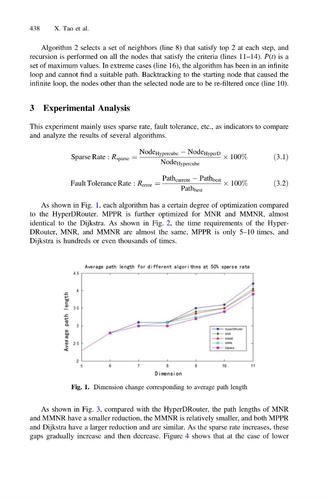
As shown in Fig. 1, each algorithm has a certain degree of optimization compared
to the HyperDRouter. MPPR is further optimized for MNR and MMNR, almost
identical to the Dijkstra. As shown in Fig. 2, the time requirements of the HyperDRouter, MNR, and MMNR are almost the same, MPPR is only 5–10 times, and
Dijkstra is hundreds or even thousands of times.
As shown in Fig. 3, compared with the HyperDRouter, the path lengths of MNR
and MMNR have a smaller reduction, the MMNR is relatively smaller, and both MPPR
and Dijkstra have a larger reduction and are similar. As the sparse rate increases, these
gaps gradually increase and then decrease. Figure 4 shows that at the case of lower
Fig. 1. Dimension change corresponding to average path length
438
X. Tao et al.