

Latency Estimation of Big Data Processing Under the MapReduce . . .
107
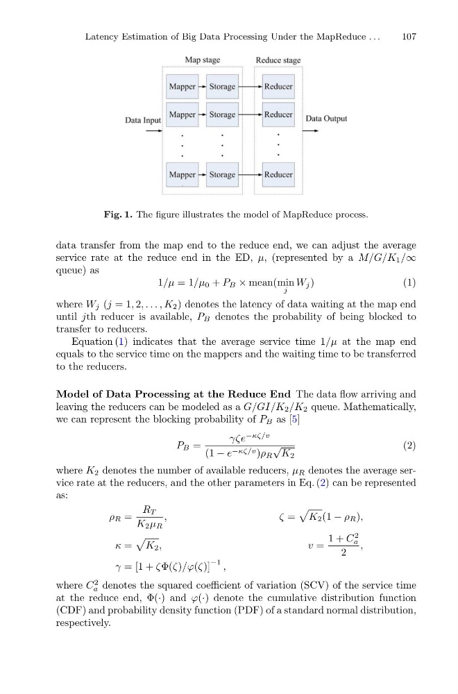
Fig. 1. The figure illustrates the model of MapReduce process.
data transfer from the map end to the reduce end, we can adjust the average
service rate at the reduce end in the ED, μ, (represented by a M/G/K 1 /∞
queue) as
1/μ = 1/μ 0 + P B × mean(min
j
W j )
(1)
where W j (j = 1, 2, . . . , K 2 ) denotes the latency of data waiting at the map end
until jth reducer is available, P B denotes the probability of being blocked to
transfer to reducers.
Equation (1) indicates that the average service time 1/μ at the map end
equals to the service time on the mappers and the waiting time to be transferred
to the reducers.
Model of Data Processing at the Reduce End The data flow arriving and
leaving the reducers can be modeled as a G/GI/K 2 /K 2 queue. Mathematically,
we can represent the blocking probability of P B as [5]
P B =
γζe
−κζ/v
(1 − e −κζ/v )ρ R
√
K 2
(2)
where K 2 denotes the number of available reducers, μ R denotes the average service rate at the reducers, and the other parameters in Eq. (2) can be represented
as:
ρ R =
R T
K 2 μ R
,
ζ =
K 2 (1 − ρ R ),
κ =
K 2 ,
v =
1 + C
2
a
2
,
γ = [1 + ζΦ(ζ)/ϕ(ζ)]
−1 ,
where C
2
a denotes the squared coefficient of variation (SCV) of the service time
at the reduce end, Φ(·) and ϕ(·) denote the cumulative distribution function
(CDF) and probability density function (PDF) of a standard normal distribution,
respectively.
107
Fig. 1. The figure illustrates the model of MapReduce process.
data transfer from the map end to the reduce end, we can adjust the average
service rate at the reduce end in the ED, μ, (represented by a M/G/K 1 /∞
queue) as
1/μ = 1/μ 0 + P B × mean(min
j
W j )
(1)
where W j (j = 1, 2, . . . , K 2 ) denotes the latency of data waiting at the map end
until jth reducer is available, P B denotes the probability of being blocked to
transfer to reducers.
Equation (1) indicates that the average service time 1/μ at the map end
equals to the service time on the mappers and the waiting time to be transferred
to the reducers.
Model of Data Processing at the Reduce End The data flow arriving and
leaving the reducers can be modeled as a G/GI/K 2 /K 2 queue. Mathematically,
we can represent the blocking probability of P B as [5]
P B =
γζe
−κζ/v
(1 − e −κζ/v )ρ R
√
K 2
(2)
where K 2 denotes the number of available reducers, μ R denotes the average service rate at the reducers, and the other parameters in Eq. (2) can be represented
as:
ρ R =
R T
K 2 μ R
,
ζ =
K 2 (1 − ρ R ),
κ =
K 2 ,
v =
1 + C
2
a
2
,
γ = [1 + ζΦ(ζ)/ϕ(ζ)]
−1 ,
where C
2
a denotes the squared coefficient of variation (SCV) of the service time
at the reduce end, Φ(·) and ϕ(·) denote the cumulative distribution function
(CDF) and probability density function (PDF) of a standard normal distribution,
respectively.