

4.2 Airy Functions and Related Functions
67
-10
-5
0
5
Re(z)
-2
-1.5
-1
-0.5
0
0.5
1
1.5
2
Im(z)
-15
-10
-5
0
5
x
-1
-0.5
0
0.5
1
y
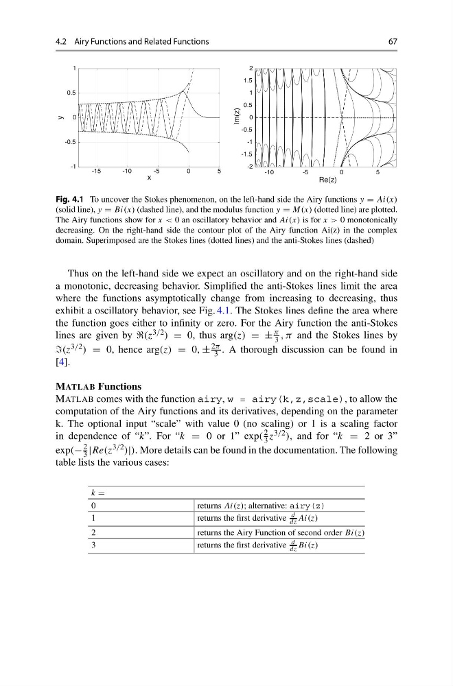
Fig. 4.1 To uncover the Stokes phenomenon, on the left-hand side the Airy functions y = Ai(x)
(solid line), y = Bi(x) (dashed line), and the modulus function y = M(x) (dotted line) are plotted.
The Airy functions show for x < 0 an oscillatory behavior and Ai(x) is for x > 0 monotonically
decreasing. On the right-hand side the contour plot of the Airy function Ai(z) in the complex
domain. Superimposed are the Stokes lines (dotted lines) and the anti-Stokes lines (dashed)
Thus on the left-hand side we expect an oscillatory and on the right-hand side
a monotonic, decreasing behavior. Simplified the anti-Stokes lines limit the area
where the functions asymptotically change from increasing to decreasing, thus
exhibit a oscillatory behavior, see Fig. 4.1. The Stokes lines define the area where
the function goes either to infinity or zero. For the Airy function the anti-Stokes
lines are given by (z 3/2 ) = 0, thus arg(z) = ±
π
3 , π and the Stokes lines by
(z 3/2 ) = 0, hence arg(z) = 0, ±
2π
3 . A thorough discussion can be found in
[4].
MATLAB Functions
MATLAB comes with the function airy, w = airy(k,z,scale), to allow the
computation of the Airy functions and its derivatives, depending on the parameter
k. The optional input “scale” with value 0 (no scaling) or 1 is a scaling factor
in dependence of “k”. For “k = 0 or 1” exp(
2
3 z 3/2 ), and for “k = 2 or 3”
exp(−
2
3 |Re(z 3/2 )|). More details can be found in the documentation. The following
table lists the various cases:
k =
0
returns Ai(z); alternative: airy(z)
1
returns the first derivative
d
dz Ai(z)
2
returns the Airy Function of second order Bi(z)
3
returns the first derivative
d
dz Bi(z)
67
-10
-5
0
5
Re(z)
-2
-1.5
-1
-0.5
0
0.5
1
1.5
2
Im(z)
-15
-10
-5
0
5
x
-1
-0.5
0
0.5
1
y
Fig. 4.1 To uncover the Stokes phenomenon, on the left-hand side the Airy functions y = Ai(x)
(solid line), y = Bi(x) (dashed line), and the modulus function y = M(x) (dotted line) are plotted.
The Airy functions show for x < 0 an oscillatory behavior and Ai(x) is for x > 0 monotonically
decreasing. On the right-hand side the contour plot of the Airy function Ai(z) in the complex
domain. Superimposed are the Stokes lines (dotted lines) and the anti-Stokes lines (dashed)
Thus on the left-hand side we expect an oscillatory and on the right-hand side
a monotonic, decreasing behavior. Simplified the anti-Stokes lines limit the area
where the functions asymptotically change from increasing to decreasing, thus
exhibit a oscillatory behavior, see Fig. 4.1. The Stokes lines define the area where
the function goes either to infinity or zero. For the Airy function the anti-Stokes
lines are given by (z 3/2 ) = 0, thus arg(z) = ±
π
3 , π and the Stokes lines by
(z 3/2 ) = 0, hence arg(z) = 0, ±
2π
3 . A thorough discussion can be found in
[4].
MATLAB Functions
MATLAB comes with the function airy, w = airy(k,z,scale), to allow the
computation of the Airy functions and its derivatives, depending on the parameter
k. The optional input “scale” with value 0 (no scaling) or 1 is a scaling factor
in dependence of “k”. For “k = 0 or 1” exp(
2
3 z 3/2 ), and for “k = 2 or 3”
exp(−
2
3 |Re(z 3/2 )|). More details can be found in the documentation. The following
table lists the various cases:
k =
0
returns Ai(z); alternative: airy(z)
1
returns the first derivative
d
dz Ai(z)
2
returns the Airy Function of second order Bi(z)
3
returns the first derivative
d
dz Bi(z)