

3.4 Associate Legendre Functions with Complex Indices
59
2
4
6
8
10
12
14
16
18
20
x
-4
-3
-2
-1
0
1
2
3
4
real
10
9
-4
-3
-2
-1
0
1
2
3
4
imag
10
9
Legendre function 1st kind
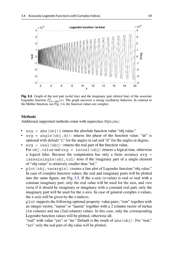
Fig. 3.5 Graph of the real part (solid line) and the imaginary part (dotted line) of the associate
Legendre function P
5
0.5+100i (x). The graph uncovers a strong oscillatory behavior. In contrast to
the Mehler function, see Fig. 3.4, the function values are complex
Methods
Additional supported methods come with superclass PQnumu:
• erg = abs(obj)): returns the absolute function value “obj.value.”
• erg = angle(obj,dr): returns the phase of the function value. “dr” is
optional with default “r,” for the angles in rad and “d” for the angles in degree.
• erg = real(obj): returns the real part of the function value.
For obj.value real erg = isreal(obj) returns a logical true, otherwise
a logical false. Because the computation has only a finite accuracy erg =
isrealsingle(obj,tol) tests if the imaginary part of a single element
of “obj.value” is relatively smaller than “tol.”
• plot(obj,varargin): creates a line plot of Legendre function “obj.value.”
In case of complex function values, the real and imaginary parts will be plotted
into the same figure, see Fig. 3.5. If the x-axis (z-value) is real or real with a
constant imaginary part, only the real value will be used for the axis, and vice
versa if it should be imaginary or imaginary with a constant real part, only the
imaginary part will be used for the x-axis. In case of general complex z-values,
the x-axis will be given by the z-indices.
plot supports the following optional property–value pairs: “row” together with
an integer vector, “numu” or “taumu” together with a 2 column vector of nu/tau
(1st column) and mu (2nd column) values. In this case, only the corresponding
Legendre function values will be plotted, otherwise all.
“real” with value “yes” or “no.” Default is the result of abs(obj). For “real,”
“yes” only the real part of obj.value will be plotted.
59
2
4
6
8
10
12
14
16
18
20
x
-4
-3
-2
-1
0
1
2
3
4
real
10
9
-4
-3
-2
-1
0
1
2
3
4
imag
10
9
Legendre function 1st kind
Fig. 3.5 Graph of the real part (solid line) and the imaginary part (dotted line) of the associate
Legendre function P
5
0.5+100i (x). The graph uncovers a strong oscillatory behavior. In contrast to
the Mehler function, see Fig. 3.4, the function values are complex
Methods
Additional supported methods come with superclass PQnumu:
• erg = abs(obj)): returns the absolute function value “obj.value.”
• erg = angle(obj,dr): returns the phase of the function value. “dr” is
optional with default “r,” for the angles in rad and “d” for the angles in degree.
• erg = real(obj): returns the real part of the function value.
For obj.value real erg = isreal(obj) returns a logical true, otherwise
a logical false. Because the computation has only a finite accuracy erg =
isrealsingle(obj,tol) tests if the imaginary part of a single element
of “obj.value” is relatively smaller than “tol.”
• plot(obj,varargin): creates a line plot of Legendre function “obj.value.”
In case of complex function values, the real and imaginary parts will be plotted
into the same figure, see Fig. 3.5. If the x-axis (z-value) is real or real with a
constant imaginary part, only the real value will be used for the axis, and vice
versa if it should be imaginary or imaginary with a constant real part, only the
imaginary part will be used for the x-axis. In case of general complex z-values,
the x-axis will be given by the z-indices.
plot supports the following optional property–value pairs: “row” together with
an integer vector, “numu” or “taumu” together with a 2 column vector of nu/tau
(1st column) and mu (2nd column) values. In this case, only the corresponding
Legendre function values will be plotted, otherwise all.
“real” with value “yes” or “no.” Default is the result of abs(obj). For “real,”
“yes” only the real part of obj.value will be plotted.