

3.2 Legendre Polynomials
35
• Oblate spheroidal functions can be computed via the function RTnm or with
the method RTnm of PQnumufun.
3.2
Legendre Polynomials
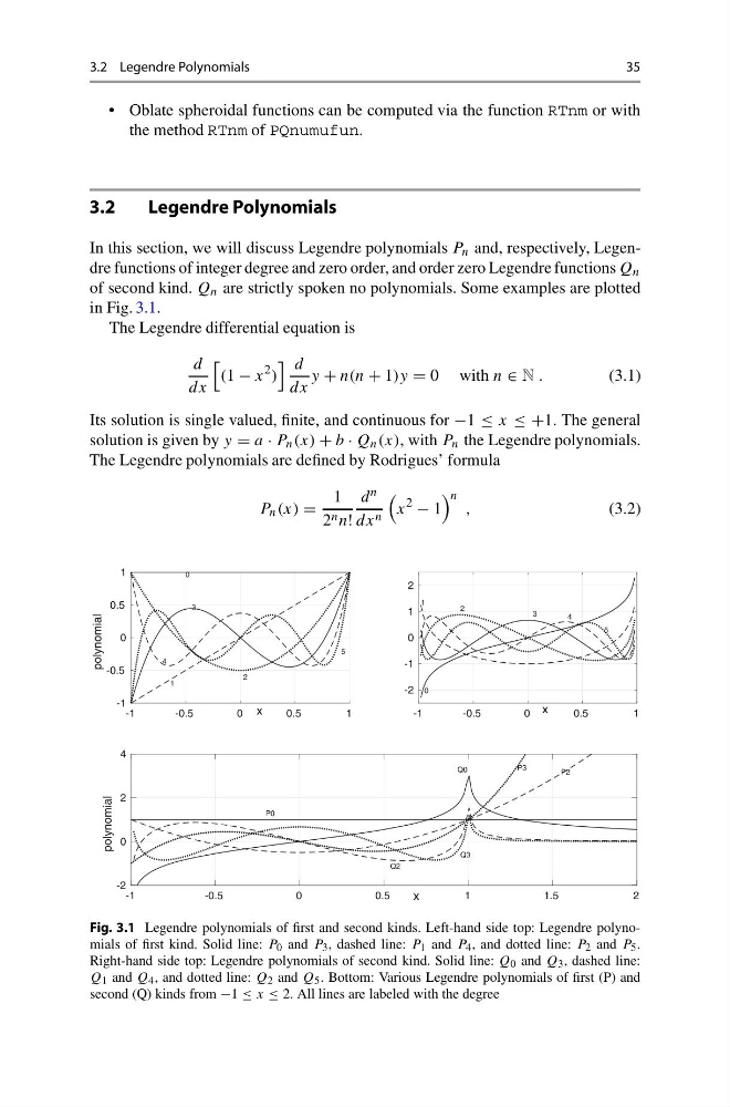
In this section, we will discuss Legendre polynomials P n and, respectively, Legendre functions of integer degree and zero order, and order zero Legendre functions Q n
of second kind. Q n are strictly spoken no polynomials. Some examples are plotted
in Fig. 3.1.
The Legendre differential equation is
d
dx
(1 − x
2 )
d
dx
y + n(n + 1)y = 0 with n ∈ N .
(3.1)
Its solution is single valued, finite, and continuous for −1 ≤ x ≤ +1. The general
solution is given by y = a · P n (x) + b · Q n (x), with P n the Legendre polynomials.
The Legendre polynomials are defined by Rodrigues’ formula
P n (x) =
1
2 n n!
d n
dx n
x
2
− 1
n
,
(3.2)
-1
-0.5
0
0.5
1
x
-1
-0.5
0
0.5
1
polynomial
-1
-0.5
0
0.5
1
x
-2
-1
0
1
2
-1
-0.5
0
0.5
1
1.5
2
x
-2
0
2
4
polynomial
0
1
3
5
2
4
1
0
4
5
P0
P2
P3
Q0
Q3
Q2
2
3
Fig. 3.1 Legendre polynomials of first and second kinds. Left-hand side top: Legendre polynomials of first kind. Solid line: P 0 and P 3 , dashed line: P 1 and P 4 , and dotted line: P 2 and P 5 .
Right-hand side top: Legendre polynomials of second kind. Solid line: Q 0 and Q 3 , dashed line:
Q 1 and Q 4 , and dotted line: Q 2 and Q 5 . Bottom: Various Legendre polynomials of first (P) and
second (Q) kinds from −1 ≤ x ≤ 2. All lines are labeled with the degree
35
• Oblate spheroidal functions can be computed via the function RTnm or with
the method RTnm of PQnumufun.
3.2
Legendre Polynomials
In this section, we will discuss Legendre polynomials P n and, respectively, Legendre functions of integer degree and zero order, and order zero Legendre functions Q n
of second kind. Q n are strictly spoken no polynomials. Some examples are plotted
in Fig. 3.1.
The Legendre differential equation is
d
dx
(1 − x
2 )
d
dx
y + n(n + 1)y = 0 with n ∈ N .
(3.1)
Its solution is single valued, finite, and continuous for −1 ≤ x ≤ +1. The general
solution is given by y = a · P n (x) + b · Q n (x), with P n the Legendre polynomials.
The Legendre polynomials are defined by Rodrigues’ formula
P n (x) =
1
2 n n!
d n
dx n
x
2
− 1
n
,
(3.2)
-1
-0.5
0
0.5
1
x
-1
-0.5
0
0.5
1
polynomial
-1
-0.5
0
0.5
1
x
-2
-1
0
1
2
-1
-0.5
0
0.5
1
1.5
2
x
-2
0
2
4
polynomial
0
1
3
5
2
4
1
0
4
5
P0
P2
P3
Q0
Q3
Q2
2
3
Fig. 3.1 Legendre polynomials of first and second kinds. Left-hand side top: Legendre polynomials of first kind. Solid line: P 0 and P 3 , dashed line: P 1 and P 4 , and dotted line: P 2 and P 5 .
Right-hand side top: Legendre polynomials of second kind. Solid line: Q 0 and Q 3 , dashed line:
Q 1 and Q 4 , and dotted line: Q 2 and Q 5 . Bottom: Various Legendre polynomials of first (P) and
second (Q) kinds from −1 ≤ x ≤ 2. All lines are labeled with the degree