

References
31
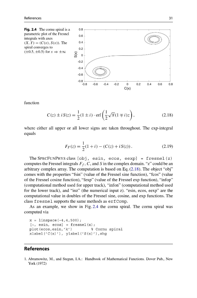
Fig. 2.4 The cornu spiral is a
parametric plot of the Fresnel
integrals with axes
(X, Y ) = (C(x), S(x)). The
spiral converges to
(±0.5, ±0.5) for x ⇒ ±∞
-0.8
-0.6
-0.4
-0.2
0
0.2
0.4
0.6
0.8
C(x)
-0.8
-0.6
-0.4
-0.2
0
0.2
0.4
0.6
0.8
S(x)
function
C(z) ± iS(z) =
1
2
(1 ± i) · erf
1
2
√
π(1 ∓ i)z
,
(2.18)
where either all upper or all lower signs are taken throughout. The exp-integral
equals
F F (z) =
1
2
(1 + i) − (C(z) + iS(z)) .
(2.19)
The SPECFUNPHYS class [obj, esin, ecos, eexp] = fresnel(z)
computes the Fresnel integrals F f , C, and S in the complex domain. “z” could be an
arbitrary complex array. The computation is based on Eq. (2.18). The object “obj”
comes with the properties “fsin” (value of the Fresnel sine function), “fcos” (value
of the Fresnel cosine function), “fexp” (value of the Fresnel exp function), “infop”
(computational method used for upper track), “infon” (computational method used
for the lower track), and “inz” (the numerical input z). “esin, ecos, eexp” are the
computational value in doubles of the Fresnel sine, cosine, and exp functions. The
class fresnel supports the same methods as erfComp.
As an example, we show in Fig. 2.4 the cornu spiral. The cornu spiral was
computed via
x = linspace(-4,4,500);
[~, esin, ecos] = fresnel(x);
plot(ecos,esin,’k’)
% Cornu spiral
xlabel(’C(x)’), ylabel(’S(x)’),shg
References
1. Abramowitz, M., and Stegun, I.A.: Handbook of Mathematical Functions. Dover Pub., New
York (1972)
31
Fig. 2.4 The cornu spiral is a
parametric plot of the Fresnel
integrals with axes
(X, Y ) = (C(x), S(x)). The
spiral converges to
(±0.5, ±0.5) for x ⇒ ±∞
-0.8
-0.6
-0.4
-0.2
0
0.2
0.4
0.6
0.8
C(x)
-0.8
-0.6
-0.4
-0.2
0
0.2
0.4
0.6
0.8
S(x)
function
C(z) ± iS(z) =
1
2
(1 ± i) · erf
1
2
√
π(1 ∓ i)z
,
(2.18)
where either all upper or all lower signs are taken throughout. The exp-integral
equals
F F (z) =
1
2
(1 + i) − (C(z) + iS(z)) .
(2.19)
The SPECFUNPHYS class [obj, esin, ecos, eexp] = fresnel(z)
computes the Fresnel integrals F f , C, and S in the complex domain. “z” could be an
arbitrary complex array. The computation is based on Eq. (2.18). The object “obj”
comes with the properties “fsin” (value of the Fresnel sine function), “fcos” (value
of the Fresnel cosine function), “fexp” (value of the Fresnel exp function), “infop”
(computational method used for upper track), “infon” (computational method used
for the lower track), and “inz” (the numerical input z). “esin, ecos, eexp” are the
computational value in doubles of the Fresnel sine, cosine, and exp functions. The
class fresnel supports the same methods as erfComp.
As an example, we show in Fig. 2.4 the cornu spiral. The cornu spiral was
computed via
x = linspace(-4,4,500);
[~, esin, ecos] = fresnel(x);
plot(ecos,esin,’k’)
% Cornu spiral
xlabel(’C(x)’), ylabel(’S(x)’),shg
References
1. Abramowitz, M., and Stegun, I.A.: Handbook of Mathematical Functions. Dover Pub., New
York (1972)