

19.2 Euler Numbers and Euler Polynomials
231
0
0.1
0.2
0.3
0.4
0.5
0.6
0.7
0.8
0.9
1
x
-0.04
-0.03
-0.02
-0.01
0
0.01
0.02
0.03
0.04
value
0
1
2
3
4
5
6
value
Bernoulli polynomial: degree = 8
Euler polynomial: degree = 8
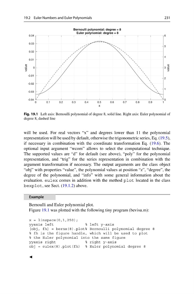
Fig. 19.1 Left axis: Bernoulli polynomial of degree 8, solid line. Right axis: Euler polynomial of
degree 8, dashed line
will be used. For real vectors “x” and degrees lower than 11 the polynomial
representation will be used by default, otherwise the trigonometric series, Eq. (19.5),
if necessary in combination with the coordinate transformation Eq. (19.6). The
optional input argument “wcom” allows to select the computational technique.
The supported values are “d” for default (see above), “poly” for the polynomial
representation, and “trig” for the series representation in combination with the
argument transformation if necessary. The output arguments are the class object
“obj” with properties “value”, the polynomial values at position “z”, “degree”, the
degree of the polynomial, and “info” with some general information about the
evaluation. eulex comes in addition with the method plot located in the class
bexplot, see Sect. (19.1.2) above.
Example
Bernoulli and Euler polynomial plot.
Figure 19.1 was plotted with the following tiny program (bevisu.m):
x = linspace(0,1,250);
yyaxis left
% left y-axis
[obj, fh] = bernx(8).plot% Bernoulli polynomial degree 8
% fh is the figure handle, which will be used to plot
% the Euler polynomial into the same figure
yyaxis right
% right y-axis
obj = eulex(8).plot(fh) % Euler polynomial degree 8
231
0
0.1
0.2
0.3
0.4
0.5
0.6
0.7
0.8
0.9
1
x
-0.04
-0.03
-0.02
-0.01
0
0.01
0.02
0.03
0.04
value
0
1
2
3
4
5
6
value
Bernoulli polynomial: degree = 8
Euler polynomial: degree = 8
Fig. 19.1 Left axis: Bernoulli polynomial of degree 8, solid line. Right axis: Euler polynomial of
degree 8, dashed line
will be used. For real vectors “x” and degrees lower than 11 the polynomial
representation will be used by default, otherwise the trigonometric series, Eq. (19.5),
if necessary in combination with the coordinate transformation Eq. (19.6). The
optional input argument “wcom” allows to select the computational technique.
The supported values are “d” for default (see above), “poly” for the polynomial
representation, and “trig” for the series representation in combination with the
argument transformation if necessary. The output arguments are the class object
“obj” with properties “value”, the polynomial values at position “z”, “degree”, the
degree of the polynomial, and “info” with some general information about the
evaluation. eulex comes in addition with the method plot located in the class
bexplot, see Sect. (19.1.2) above.
Example
Bernoulli and Euler polynomial plot.
Figure 19.1 was plotted with the following tiny program (bevisu.m):
x = linspace(0,1,250);
yyaxis left
% left y-axis
[obj, fh] = bernx(8).plot% Bernoulli polynomial degree 8
% fh is the figure handle, which will be used to plot
% the Euler polynomial into the same figure
yyaxis right
% right y-axis
obj = eulex(8).plot(fh) % Euler polynomial degree 8