

16.3 Oscillator Systems
207
and can be used to compute the expectation value of an operator ˆ
A = T r[ ˆ
ρ ˆ
A],
with T r the trace. We now define the Wigner function as [3, 6]
W (q, p) =
1
π ¯
h
dy − y| ˆ
ρ|q + y exp(2ipy/ ¯
h) ,
(16.22a)
and thus equivalently
W (q, p) =
1
π ¯
h
dyψ(x + y)ψ
† (x − y) exp(2ipy/ ¯
h).
(16.22b)
Integrating the Wigner function in Mock phase space over the momenta results in
the probability of presence in coordinate space, and vice versa, integrating over the
coordinate space will lead to the probability of presence in momentum space:
W (q, p)dp = ||q|ψ 2
W (q, p)dq = ||p|ψ 2 .
(16.23)
Additional properties of the Wigner function in phase space can be found in [3] and
many text books about quantum optics.
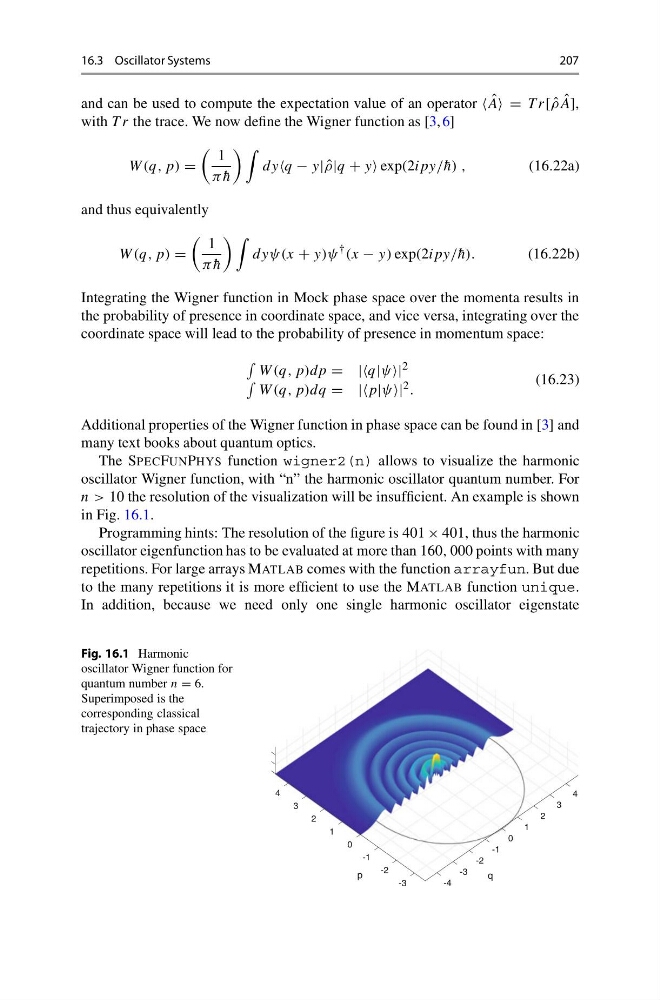
The SPECFUNPHYS function wigner2(n) allows to visualize the harmonic
oscillator Wigner function, with “n” the harmonic oscillator quantum number. For
n > 10 the resolution of the visualization will be insufficient. An example is shown
in Fig. 16.1.
Programming hints: The resolution of the figure is 401 × 401, thus the harmonic
oscillator eigenfunction has to be evaluated at more than 160, 000 points with many
repetitions. For large arrays MATLAB comes with the function arrayfun. But due
to the many repetitions it is more efficient to use the MATLAB function unique.
In addition, because we need only one single harmonic oscillator eigenstate
Fig. 16.1 Harmonic
oscillator Wigner function for
quantum number n = 6.
Superimposed is the
corresponding classical
trajectory in phase space
4
4
3
3
2
2
1
1
p
q
0
0
-1
-1
-2
-2
-3
-4
-3
207
and can be used to compute the expectation value of an operator ˆ
A = T r[ ˆ
ρ ˆ
A],
with T r the trace. We now define the Wigner function as [3, 6]
W (q, p) =
1
π ¯
h
dy − y| ˆ
ρ|q + y exp(2ipy/ ¯
h) ,
(16.22a)
and thus equivalently
W (q, p) =
1
π ¯
h
dyψ(x + y)ψ
† (x − y) exp(2ipy/ ¯
h).
(16.22b)
Integrating the Wigner function in Mock phase space over the momenta results in
the probability of presence in coordinate space, and vice versa, integrating over the
coordinate space will lead to the probability of presence in momentum space:
W (q, p)dp = ||q|ψ 2
W (q, p)dq = ||p|ψ 2 .
(16.23)
Additional properties of the Wigner function in phase space can be found in [3] and
many text books about quantum optics.
The SPECFUNPHYS function wigner2(n) allows to visualize the harmonic
oscillator Wigner function, with “n” the harmonic oscillator quantum number. For
n > 10 the resolution of the visualization will be insufficient. An example is shown
in Fig. 16.1.
Programming hints: The resolution of the figure is 401 × 401, thus the harmonic
oscillator eigenfunction has to be evaluated at more than 160, 000 points with many
repetitions. For large arrays MATLAB comes with the function arrayfun. But due
to the many repetitions it is more efficient to use the MATLAB function unique.
In addition, because we need only one single harmonic oscillator eigenstate
Fig. 16.1 Harmonic
oscillator Wigner function for
quantum number n = 6.
Superimposed is the
corresponding classical
trajectory in phase space
4
4
3
3
2
2
1
1
p
q
0
0
-1
-1
-2
-2
-3
-4
-3