

12.2 Fundamental Equations and Computation
155
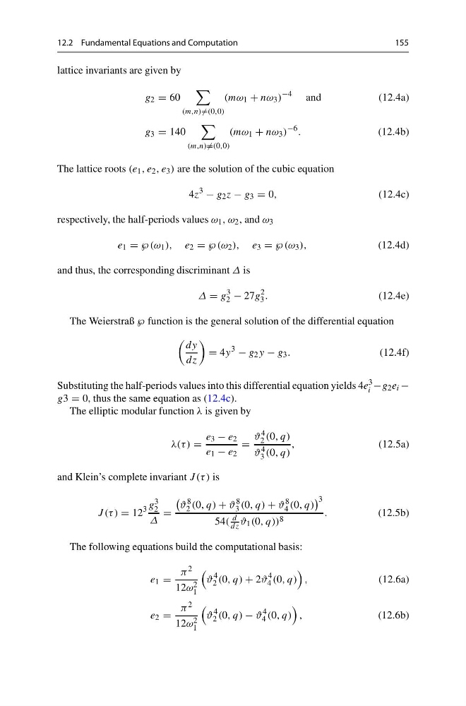
lattice invariants are given by
g 2 = 60
(m,n) =(0,0)
(mω 1 + nω 3 )
−4
and
(12.4a)
g 3 = 140
(m,n) =(0,0)
(mω 1 + nω 3 )
−6 .
(12.4b)
The lattice roots (e 1 , e 2 , e 3 ) are the solution of the cubic equation
4z
3
− g 2 z − g 3 = 0,
(12.4c)
respectively, the half-periods values ω 1 , ω 2 , and ω 3
e 1 = ℘ (ω 1 ), e 2 = ℘ (ω 2 ), e 3 = ℘ (ω 3 ),
(12.4d)
and thus, the corresponding discriminant Δ is
Δ = g
3
2 − 27g
2
3 .
(12.4e)
The Weierstraß ℘ function is the general solution of the differential equation
dy
dz
= 4y
3
− g 2 y − g 3 .
(12.4f)
Substituting the half-periods values into this differential equation yields 4e
3
i −g 2 e i −
g3 = 0, thus the same equation as (12.4c).
The elliptic modular function λ is given by
λ(τ ) =
e 3 − e 2
e 1 − e 2
=
ϑ 4
2 (0, q)
ϑ 4
3 (0, q)
,
(12.5a)
and Klein’s complete invariant J (τ ) is
J (τ ) = 12
3 g 3
2
Δ
=
ϑ
8
2 (0, q) + ϑ
8
3 (0, q) + ϑ
8
4 (0, q)
3
54(
d
dz ϑ 1 (0, q)) 8
.
(12.5b)
The following equations build the computational basis:
e 1 =
π 2
12ω 2
1
ϑ
4
2 (0, q) + 2ϑ
4
4 (0, q)
,
(12.6a)
e 2 =
π 2
12ω 2
1
ϑ
4
2 (0, q) − ϑ
4
4 (0, q)
,
(12.6b)
155
lattice invariants are given by
g 2 = 60
(m,n) =(0,0)
(mω 1 + nω 3 )
−4
and
(12.4a)
g 3 = 140
(m,n) =(0,0)
(mω 1 + nω 3 )
−6 .
(12.4b)
The lattice roots (e 1 , e 2 , e 3 ) are the solution of the cubic equation
4z
3
− g 2 z − g 3 = 0,
(12.4c)
respectively, the half-periods values ω 1 , ω 2 , and ω 3
e 1 = ℘ (ω 1 ), e 2 = ℘ (ω 2 ), e 3 = ℘ (ω 3 ),
(12.4d)
and thus, the corresponding discriminant Δ is
Δ = g
3
2 − 27g
2
3 .
(12.4e)
The Weierstraß ℘ function is the general solution of the differential equation
dy
dz
= 4y
3
− g 2 y − g 3 .
(12.4f)
Substituting the half-periods values into this differential equation yields 4e
3
i −g 2 e i −
g3 = 0, thus the same equation as (12.4c).
The elliptic modular function λ is given by
λ(τ ) =
e 3 − e 2
e 1 − e 2
=
ϑ 4
2 (0, q)
ϑ 4
3 (0, q)
,
(12.5a)
and Klein’s complete invariant J (τ ) is
J (τ ) = 12
3 g 3
2
Δ
=
ϑ
8
2 (0, q) + ϑ
8
3 (0, q) + ϑ
8
4 (0, q)
3
54(
d
dz ϑ 1 (0, q)) 8
.
(12.5b)
The following equations build the computational basis:
e 1 =
π 2
12ω 2
1
ϑ
4
2 (0, q) + 2ϑ
4
4 (0, q)
,
(12.6a)
e 2 =
π 2
12ω 2
1
ϑ
4
2 (0, q) − ϑ
4
4 (0, q)
,
(12.6b)