

8.2 Method of Computation
117
2 F 1 (a, a +
1
2
; 2a; z) = 2
2a−1 (1 − z)
−
1
2
1 +
√
1 − z
1−2a
, (8.12e)
2 F 1 (b, b +
1
2
; 2b; z) = 2
2b−1 (1 − z)
−
1
2
1 +
√
1 − z
1−2b
.
2 F 1 (
1
2
, 1;
3
2
; z
2 ) =
1
2 z
ln
1 + z
1 − z
,
(8.13a)
2 F 1 (
1
2
,
1
2
;
3
2
; z
2 ) =
1
z
arcsin(z)
(8.13b)
2 F 1 (
1 + n
2
,
1 − n
2
;
3
2
; z
2 ) =
sin (n arcsin(z))
n z
,
(8.13c)
2 F 1 (1 +
n
2
, 1 −
n
2
;
3
2
; z
2 ) =
sin (n arcsin(z))
n z
√
1 − z 2
,
(8.13d)
2 F 1 (
n
2
, −
n
2
;
1
2
; z
2 ) = cos (n arcsin(z)) ,
(8.13e)
2 F 1 (
1 + n
2
,
1 − n
2
;
1
2
; z
2 ) =
cos (n arcsin(z))
√
1 − z 2
,
(8.13f)
and
2 F 1 (
1
2
,
1
2
; 1; z
2 ) =
2
π
K(z),
(8.13g)
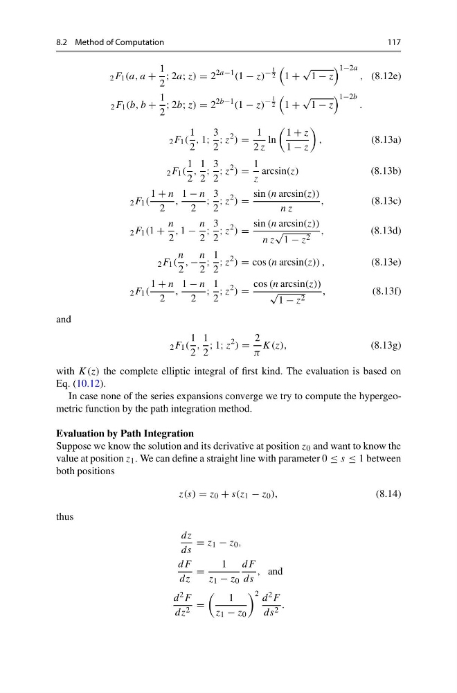
with K(z) the complete elliptic integral of first kind. The evaluation is based on
Eq. (10.12).
In case none of the series expansions converge we try to compute the hypergeometric function by the path integration method.
Evaluation by Path Integration
Suppose we know the solution and its derivative at position z 0 and want to know the
value at position z 1 . We can define a straight line with parameter 0 ≤ s ≤ 1 between
both positions
z(s) = z 0 + s(z 1 − z 0 ),
(8.14)
thus
dz
ds
= z 1 − z 0 ,
dF
dz
=
1
z 1 − z 0
dF
ds
, and
d 2 F
dz 2 =
1
z 1 − z 0
2 d 2 F
ds 2 .
117
2 F 1 (a, a +
1
2
; 2a; z) = 2
2a−1 (1 − z)
−
1
2
1 +
√
1 − z
1−2a
, (8.12e)
2 F 1 (b, b +
1
2
; 2b; z) = 2
2b−1 (1 − z)
−
1
2
1 +
√
1 − z
1−2b
.
2 F 1 (
1
2
, 1;
3
2
; z
2 ) =
1
2 z
ln
1 + z
1 − z
,
(8.13a)
2 F 1 (
1
2
,
1
2
;
3
2
; z
2 ) =
1
z
arcsin(z)
(8.13b)
2 F 1 (
1 + n
2
,
1 − n
2
;
3
2
; z
2 ) =
sin (n arcsin(z))
n z
,
(8.13c)
2 F 1 (1 +
n
2
, 1 −
n
2
;
3
2
; z
2 ) =
sin (n arcsin(z))
n z
√
1 − z 2
,
(8.13d)
2 F 1 (
n
2
, −
n
2
;
1
2
; z
2 ) = cos (n arcsin(z)) ,
(8.13e)
2 F 1 (
1 + n
2
,
1 − n
2
;
1
2
; z
2 ) =
cos (n arcsin(z))
√
1 − z 2
,
(8.13f)
and
2 F 1 (
1
2
,
1
2
; 1; z
2 ) =
2
π
K(z),
(8.13g)
with K(z) the complete elliptic integral of first kind. The evaluation is based on
Eq. (10.12).
In case none of the series expansions converge we try to compute the hypergeometric function by the path integration method.
Evaluation by Path Integration
Suppose we know the solution and its derivative at position z 0 and want to know the
value at position z 1 . We can define a straight line with parameter 0 ≤ s ≤ 1 between
both positions
z(s) = z 0 + s(z 1 − z 0 ),
(8.14)
thus
dz
ds
= z 1 − z 0 ,
dF
dz
=
1
z 1 − z 0
dF
ds
, and
d 2 F
dz 2 =
1
z 1 − z 0
2 d 2 F
ds 2 .