

108
7 Coulomb Wave Functions
and for parameterization (b),
rhotp =
√
1 + γ l(l + 1) − 1
γ
,
(7.19b)
– “sl” is the Coulomb phase sl = arg γ (l + 1 + iγ ) for parameterization (a).
The output variable “result” equals “obj.value.”
Evaluation of the Partial Wave Expansion of the Coulomb Field
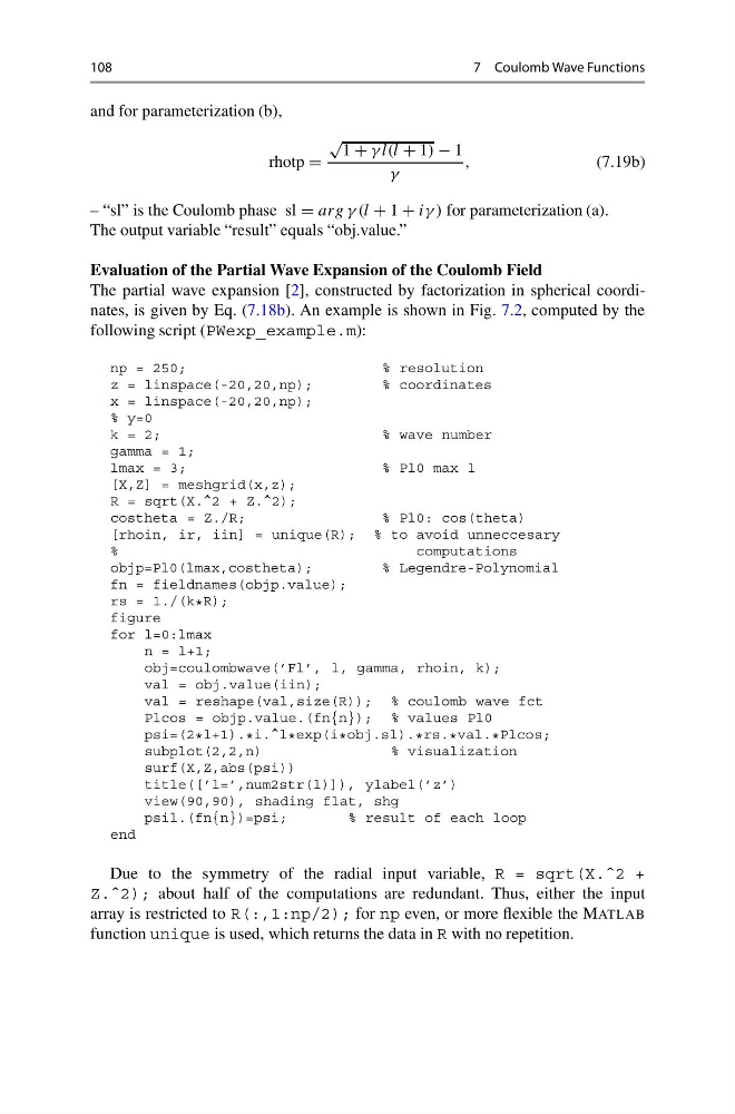
The partial wave expansion [2], constructed by factorization in spherical coordinates, is given by Eq. (7.18b). An example is shown in Fig. 7.2, computed by the
following script (PWexp_example.m):
np = 250;
% resolution
z = linspace(-20,20,np);
% coordinates
x = linspace(-20,20,np);
% y=0
k = 2;
% wave number
gamma = 1;
lmax = 3;
% Pl0 max l
[X,Z] = meshgrid(x,z);
R = sqrt(X.^2 + Z.^2);
costheta = Z./R;
% Pl0: cos(theta)
[rhoin, ir, iin] = unique(R); % to avoid unneccesary
%
computations
objp=Pl0(lmax,costheta);
% Legendre-Polynomial
fn = fieldnames(objp.value);
rs = 1./(k * R);
figure
for l=0:lmax
n = l+1;
obj=coulombwave(’Fl’, l, gamma, rhoin, k);
val = obj.value(iin);
val = reshape(val,size(R)); % coulomb wave fct
Plcos = objp.value.(fn{n}); % values Pl0
psi=(2 * l+1). * i.^l * exp(i * obj.sl). * rs. * val. * Plcos;
subplot(2,2,n)
% visualization
surf(X,Z,abs(psi))
title([’l=’,num2str(l)]), ylabel(’z’)
view(90,90), shading flat, shg
psil.(fn{n})=psi;
% result of each loop
end
Due to the symmetry of the radial input variable, R = sqrt(X.ˆ2 +
Z.ˆ2); about half of the computations are redundant. Thus, either the input
array is restricted to R(:,1:np/2); for np even, or more flexible the MATLAB
function unique is used, which returns the data in R with no repetition.
7 Coulomb Wave Functions
and for parameterization (b),
rhotp =
√
1 + γ l(l + 1) − 1
γ
,
(7.19b)
– “sl” is the Coulomb phase sl = arg γ (l + 1 + iγ ) for parameterization (a).
The output variable “result” equals “obj.value.”
Evaluation of the Partial Wave Expansion of the Coulomb Field
The partial wave expansion [2], constructed by factorization in spherical coordinates, is given by Eq. (7.18b). An example is shown in Fig. 7.2, computed by the
following script (PWexp_example.m):
np = 250;
% resolution
z = linspace(-20,20,np);
% coordinates
x = linspace(-20,20,np);
% y=0
k = 2;
% wave number
gamma = 1;
lmax = 3;
% Pl0 max l
[X,Z] = meshgrid(x,z);
R = sqrt(X.^2 + Z.^2);
costheta = Z./R;
% Pl0: cos(theta)
[rhoin, ir, iin] = unique(R); % to avoid unneccesary
%
computations
objp=Pl0(lmax,costheta);
% Legendre-Polynomial
fn = fieldnames(objp.value);
rs = 1./(k * R);
figure
for l=0:lmax
n = l+1;
obj=coulombwave(’Fl’, l, gamma, rhoin, k);
val = obj.value(iin);
val = reshape(val,size(R)); % coulomb wave fct
Plcos = objp.value.(fn{n}); % values Pl0
psi=(2 * l+1). * i.^l * exp(i * obj.sl). * rs. * val. * Plcos;
subplot(2,2,n)
% visualization
surf(X,Z,abs(psi))
title([’l=’,num2str(l)]), ylabel(’z’)
view(90,90), shading flat, shg
psil.(fn{n})=psi;
% result of each loop
end
Due to the symmetry of the radial input variable, R = sqrt(X.ˆ2 +
Z.ˆ2); about half of the computations are redundant. Thus, either the input
array is restricted to R(:,1:np/2); for np even, or more flexible the MATLAB
function unique is used, which returns the data in R with no repetition.