

6.1 Confluent Hypergeometric Function of 1st and 2nd Kind
95
Computational Techniques
The computation of the hypergeometric function 2 F 0 (a, b; ; z) is based on
Eq. (6.10b), except for negative integer parameters a or b in which case the series
expansion (6.12) becomes finite. Similar, the confluent hypergeometric function
U(a, b, z) becomes a finite polynomial for a or a − b + 1 negative integers
(· · · , −2, −1, 0), Eq. (6.10b), and for
U(a, a + 1, z) = z
−a .
(6.13)
In case U(a, b, z) is neither a finite polynomial nor b = a + 1 the evaluation is
based either on Eq. (6.10a), the path integral method, or an approximation ansatz.
Equation (6.10a) is given by the sum of two terms. Even if both summands are
converged the total sum could be meaningless due to the finite accuracy of numbers.
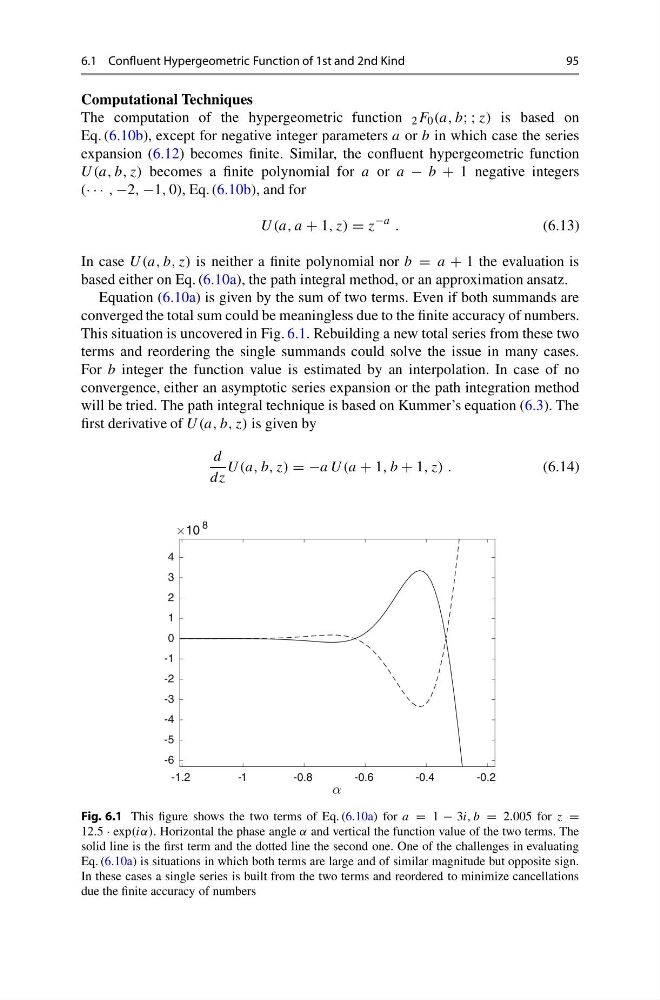
This situation is uncovered in Fig. 6.1. Rebuilding a new total series from these two
terms and reordering the single summands could solve the issue in many cases.
For b integer the function value is estimated by an interpolation. In case of no
convergence, either an asymptotic series expansion or the path integration method
will be tried. The path integral technique is based on Kummer’s equation (6.3). The
first derivative of U(a, b, z) is given by
d
dz
U(a, b, z) = −a U(a + 1, b + 1, z) .
(6.14)
-1.2
-1
-0.8
-0.6
-0.4
-0.2
-6
-5
-4
-3
-2
-1
0
1
2
3
4
10
8
Fig. 6.1 This figure shows the two terms of Eq. (6.10a) for a = 1 − 3i, b = 2.005 for z =
12.5 · exp(iα). Horizontal the phase angle α and vertical the function value of the two terms. The
solid line is the first term and the dotted line the second one. One of the challenges in evaluating
Eq. (6.10a) is situations in which both terms are large and of similar magnitude but opposite sign.
In these cases a single series is built from the two terms and reordered to minimize cancellations
due the finite accuracy of numbers
95
Computational Techniques
The computation of the hypergeometric function 2 F 0 (a, b; ; z) is based on
Eq. (6.10b), except for negative integer parameters a or b in which case the series
expansion (6.12) becomes finite. Similar, the confluent hypergeometric function
U(a, b, z) becomes a finite polynomial for a or a − b + 1 negative integers
(· · · , −2, −1, 0), Eq. (6.10b), and for
U(a, a + 1, z) = z
−a .
(6.13)
In case U(a, b, z) is neither a finite polynomial nor b = a + 1 the evaluation is
based either on Eq. (6.10a), the path integral method, or an approximation ansatz.
Equation (6.10a) is given by the sum of two terms. Even if both summands are
converged the total sum could be meaningless due to the finite accuracy of numbers.
This situation is uncovered in Fig. 6.1. Rebuilding a new total series from these two
terms and reordering the single summands could solve the issue in many cases.
For b integer the function value is estimated by an interpolation. In case of no
convergence, either an asymptotic series expansion or the path integration method
will be tried. The path integral technique is based on Kummer’s equation (6.3). The
first derivative of U(a, b, z) is given by
d
dz
U(a, b, z) = −a U(a + 1, b + 1, z) .
(6.14)
-1.2
-1
-0.8
-0.6
-0.4
-0.2
-6
-5
-4
-3
-2
-1
0
1
2
3
4
10
8
Fig. 6.1 This figure shows the two terms of Eq. (6.10a) for a = 1 − 3i, b = 2.005 for z =
12.5 · exp(iα). Horizontal the phase angle α and vertical the function value of the two terms. The
solid line is the first term and the dotted line the second one. One of the challenges in evaluating
Eq. (6.10a) is situations in which both terms are large and of similar magnitude but opposite sign.
In these cases a single series is built from the two terms and reordered to minimize cancellations
due the finite accuracy of numbers